18. Root Finding
In this chapter we cover how to find the “root” of a function \(f(x)\). The root of this function is the value of \(x\) where the function In other words, we are looking for the value of \(x\) where the function, if we plotted it, crosses the horizontal x-axis. At this value of \(x\) the function value is \(f(x) = 0\).
18.1. First Steps
import numpy as np
import matplotlib.pyplot as plt
#
import time  # Imports system time module to time your script
#
plt.close('all')  # close all open figures
Define am example function for which we calculate the root. Let us use this function:
We first program this function using the def keyword in Python. Do not
forget to also load the numpy library first.
def f_func(x):
    # Function: f(x)
    fx = np.log(x) - np.exp(-x)
    return fx
We next plot the function.
xmin = 1
xmax = 3
xv  = np.arange(xmin, xmax, (xmax - xmin)/200.0)
fxv = np.zeros(len(xv),float) # define column vector
for i in range(len(xv)):
    fxv[i] = f_func(xv[i])
fig, ax = plt.subplots()
ax.plot(xv, fxv)
ax.plot(xv, np.zeros(len(xv)))
# Create a title with a red, bold/italic font
plt.show()
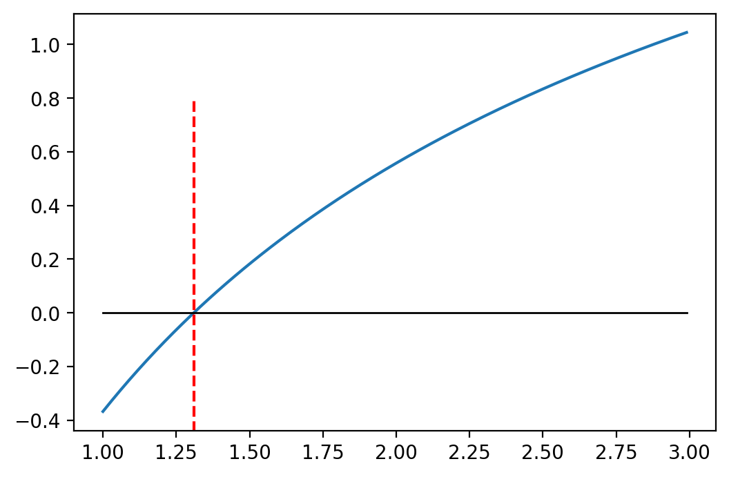
We clearly see that the “root” of the function is somewhere near an x of 1.25 to 1.35.
18.2. Newton-Raphson
Fig. 18.1 presents an illustration of the Newton-Raphson algorithm.
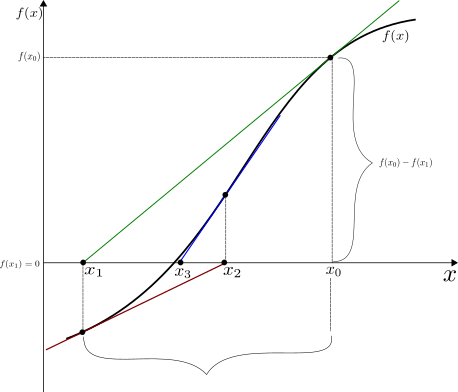
Fig. 18.1 The Newton-Raphson Algorithm
We start with an initial guess \(x_0\). The slope of the tangent line through the initial guess can be defined as rise \(f(x_0) - 0\) over run \(x_0-x_1\) or:
where \(x_1\) is the point where the tangent line crosses the x-axis. This point has coordinates \(x_1\) and \(y_1 = 0\). Our goal is to find the value of \(x_1\).
Since this line is a tangent line, we can also write its slope as the derivative of function \(f\) that is: \(f'(x)\). We now set the derivative equal to the expression for the slope:
\[f'(x_0) = slope = \frac{f(x_0)-0}{x_0-x_1},\]
which we can now use to solve for the value of \(x_1\):
We next put a tangent line through the value of \(f(x_1)\) and search where this tangent line crosses the x-axis at point \(x_2\) in Fig. 18.1. This results in
\[f'(x_1) = slope = \frac{f(x_1)-0}{x_1-x_2},\]
which we can now use to solve for the value of \(x_2\):
Note
We can now repeat this successively using the iterative procedure:
In order for this function to work well we need to be able to calculate the derivative of the function around the root point and preferably over the entire domain of the function.
In the following code we “hand in” a function ftn which is a user specified
function. This function needs to return 2! values:
the functional value \(f(x)\), and
the value of the first derivative \(f'(x)\).
def newtonraphson(ftn, x0, tol = 1e-9, maxiter = 100):
    # Newton_Raphson algorithm for solving ftn(x)[1] == 0
    # we assume that ftn is a function of a single
    # variable that returns the function value and
    # the first derivative as a vector of length 2
    #
    # x0 is the initial guess at the root
    # the algorithm terminates when the function
    # value is within distance tol of 0, or the
    # number of iterations exceeds maxiter

    x = x0

    # Evaluate user supplied function at starting value
    fxv = ftn(x)
    fx = fxv[0]   # function value f(x)
    d_fx = fxv[1]  # derivative value f'(x)

    jiter =  0

    # Continue iterating until stopping conditions are met
    while ((abs(fx) > tol) and (jiter < maxiter)):

        # Newton-Raphson iterative formula
        x = x - fx/d_fx

        # Update function and derivative value
        fxv = ftn(x)
        fx = fxv[0]   # new function value f(x)
        d_fx = fxv[1]  # new derivative value f'(x)

        jiter =  jiter + 1
        print("At iteration: {} the value of x is {}:" \
          .format(jiter, x))

    # Output depends on success of algorithm
    if (abs(fx) > tol):
        print("Algorithm failed to converge")
        return None
    else:
        print("fx = ", fx)
        print("Algorithm converged")
        return x
In order to implement this method we will need the derivative value of the function. Calculus to the rescue. Let us take the derivative of our function. Here is the function:
And here is its derivative. Check your calculus books if you forgot how to do this!
which can be written as
So let us define our example function from the beginning of the chapter again but this time we return both, the functional value and the value of the first derivate (i.e., the gradient).
def f_func1(x):
    # Function: f(x)
    fx = np.log(x) - np.exp(-x)

    # Derivative of function: f'(x)
    d_fx = 1.0/x + np.exp(-x)

    return np.array([fx, d_fx])
We next calculate the root of the function func1 calling the
newtonraphson algorithm.
myRoot = newtonraphson(f_func1, 2.0)

print('--------------------------------')
print('My Root is at {:8.4f}'.format(myRoot))
print('--------------------------------')
At iteration: 1 the value of x is 1.122019645309717:
At iteration: 2 the value of x is 1.2949969704390394:
At iteration: 3 the value of x is 1.3097090626648604:
At iteration: 4 the value of x is 1.309799582422906:
At iteration: 5 the value of x is 1.3097995858041505:
fx =  -5.551115123125783e-17
Algorithm converged
--------------------------------
My Root is at   1.3098
--------------------------------
We can now plot the function again. Using axvline we can mark the root of
the function in the graph.
fig, ax = plt.subplots()
ax.plot(xv, fxv)
ax.plot(xv, np.zeros(len(xv)), 'k', linewidth = 1)
ax.axvline(x = myRoot, ymin=-0.3, ymax=0.8, color='r', linestyle='--')
# Create a title with a red, bold/italic font
plt.show()
Warning
The Newton-Raphson algorithm has two shortcomings:
It requires that the function is differentiable. For non-differential functions (i.e., functions with “kinks” or steps) this algorithm will not work.
It is sensitive to starting values. If a bad starting value is chosen and if the function exhibits “flat” spots, the algorithm will not converge.
Fig. 18.2 presents an illustration of the Newton-Raphson algorithm when the starting value is chosen far from the root point in the “flat” area of the function. In this case the tangent line crosses the z-axis at a very distant point from the root we are looking for and might not converge or only converge very slowly.
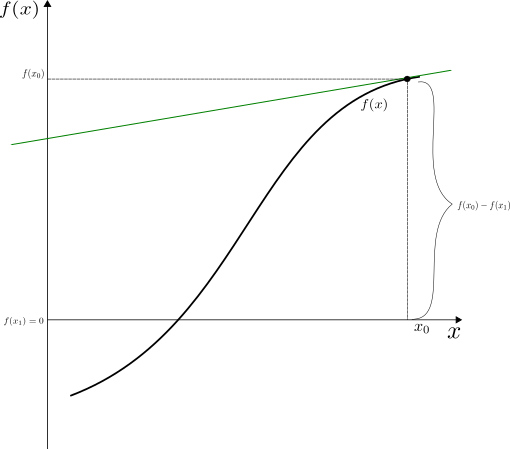
Fig. 18.2 The Newton-Raphson Algorithm with Bad Starting Value
18.3. Secant Method
As pointed out above, in order to use the Newton-Raphson method we need to be able to calculate the derivative \(f'(x)\) of the function. If this is computationally expensive or maybe even impossible, we can use the secant method which only requires that the function is continuous. That is, it does not have to be differentiable over its domain.
In this case we start with two starting values or initial guesses, \(x_0\) and \(x_1\) and put a line through the functional values \(f(x_0)\) and \(f(x_1)\). The advantage of this method is that we do not have to calculate the first derivative of the function.
Fig. 18.3 presents an illustration of the Secant method. The green line is formed using the functional values of the two starting guesses ,:math:x_0 and \(x_1\). The closer the two starting values are to each other the more the green secant (line) will resemble the tangent line in Fig. 18.1 that was used in the Newton-Raphson algorithm above.
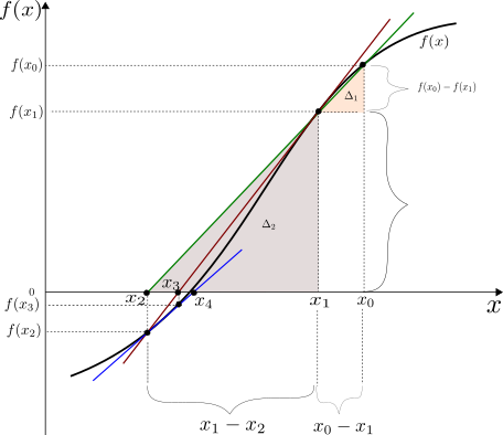
Fig. 18.3 The Secant Algorithm
The algorithm then proceeds in finding point \(x_2\) where the green secant crosses the x-axis. The slope of the secant line can be calculated in two ways using the rise-over-run method. We can first express the slope as:
And similarly we can use a second triangle (rise over run) and express the slope as:
We can now set the two expressions equal to each other
and since we have \(x_0,x_1,f(x_0),\) and \(f(x_1)\) we can solve for \(x_2\).
The iterative procedure can be written as:
Note
Keep in mind that if \(x_0\) and \(x_1\) are close together then:
So that the Secant method is really an approximation of the Newton-Raphson method, where we substitute \(\frac{f(x_n)-f(x_{n-1})}{x_n-x_{n-1}}\) for \(f'(x)\).
In this sense we can also write the iterative procedure of the Secant method as:
def secant(ftn, x0, x1, tol = 1e-9, maxiter = 100):
    # Secant algorithm for solving ftn(x) == 0
    # we assume that ftn is a function of a
    # single variable that returns the function value
    #
    # x0 and x1 are the initial guesses around the root
    # the algorithm terminates when the function
    # value is within distance
    # tol of 0, or the number of iterations exceeds max.iter

    fx0 = ftn(x0)
    fx1 = ftn(x1)
    jiter =  0

    # continue iterating until stopping conditions are met
    while ((abs(fx1) > tol) and (jiter < maxiter)):
        x  = x1 - fx1 * (x1-x0)/(fx1 - fx0)
        fx0 = ftn(x1)
        fx1 = ftn(x)
        x0  = x1
        x1  = x
        jiter =  jiter + 1
        print("At iteration: {} the value of x is: {}" \
          .format(jiter, x))

    # output depends on success of algorithm
    if (abs(fx1) > tol):
        print("Algorithm failed to converge")
        return None
    else:
       print("Algorithm converged")
       return x
We next calculate the root point using the secant method:
myRoot = secant(f_func, 1,2)
print('--------------------------------')
print('My Root is at {:8.4f}'.format(myRoot))
print('--------------------------------')
At iteration: 1 the value of x is: 1.3974104821696125
At iteration: 2 the value of x is: 1.2854761201506528
At iteration: 3 the value of x is: 1.310676758082541
At iteration: 4 the value of x is: 1.3098083980193003
At iteration: 5 the value of x is: 1.3097995826147546
At iteration: 6 the value of x is: 1.309799585804162
Algorithm converged
--------------------------------
My Root is at   1.3098
--------------------------------
18.4. Bisection
The Newton-Raphson as well as the Secant method are not guaranteed to work. The bisection method is the most robust method, but it is slow. We start with two values \(x_l < x_r\) which bracket the root of the function. It therefore must hold that \(f(x_l) \times f(x_r) < 0\). The algorithm then repeatedly brackets around the root in the following systematic way:
Note
if \(x_r - x_l \le \epsilon\) then stop
calculate midpoint: \(x_m = (x_l+x_r)/2\)
if \(f(x_m)==0\) stop
if \(f(x_l) \times f(x_m) < 0\) then set \(x_r = x_m\) otherwise \(x_l=x_m\)
go back to step 1
Fig. 18.4 demonstrates the Bisection algorithm. In the figure we demonstrate the first case in step 4 above, where \(f(x_l) \times f(x_m) < 0\) so that we move the right bracket inwards.

Fig. 18.4 The Bisection Algorithm
Here is the algorithm of the Bisection method:
def bisection(ftn, xl, xr, tol = 1e-9):
    # applies the bisection algorithm to find x
    # such that ftn(x) == 0
    # we assume that ftn is a function of a single variable
    #
    # x.l and x.r must bracket the fixed point, that is
    # x.l < x.r and ftn(x.l) * ftn(x.r) < 0
    #
    # the algorithm iteratively refines
    # x.l and x.r and terminates when
    # x.r - x.l <= tol

    # check inputs
    if (xl >= xr):
        print("error: xl >= xr")
        return None

    fl = ftn(xl)
    fr = ftn(xr)

    if (fl == 0):
        return xl
    elif (fr == 0):
        return xr
    elif (fl * fr > 0):
        print("error: ftn(xl) * ftn(xr) > 0")
        return None

    # successively refine x.l and x.r
    n = 0
    while ((xr - xl) > tol):
        xm = (xl + xr)/2.0
        fm = ftn(xm)
        if (fm == 0):
            return fm
        elif (fl * fm < 0):
            xr = xm
            fr = fm
        else:
            xl = xm
            fl = fm
        n = n + 1
        print("at iteration: {} the root lies between {} and {}" \
            .format(n, xl, xr))
    # return (approximate) root
    return (xl + xr)/2.0
We next calculate the root of the function calling ‘bisection’ method:
myRoot = bisection(f_func, 1,2)

print('--------------------------------')
print('My Root is at {:8.4f}'.format(myRoot))
print('--------------------------------')
at iteration: 1 the root lies between 1 and 1.5
at iteration: 2 the root lies between 1.25 and 1.5
at iteration: 3 the root lies between 1.25 and 1.375
at iteration: 4 the root lies between 1.25 and 1.3125
at iteration: 5 the root lies between 1.28125 and 1.3125
at iteration: 6 the root lies between 1.296875 and 1.3125
at iteration: 7 the root lies between 1.3046875 and 1.3125
at iteration: 8 the root lies between 1.30859375 and 1.3125
at iteration: 9 the root lies between 1.30859375 and 1.310546875
at iteration: 10 the root lies between 1.3095703125 and 1.310546875
at iteration: 11 the root lies between 1.3095703125 and 1.31005859375
at iteration: 12 the root lies between 1.3095703125 and 1.309814453125
at iteration: 13 the root lies between 1.3096923828125 and
1.309814453125
at iteration: 14 the root lies between 1.30975341796875 and
1.309814453125
at iteration: 15 the root lies between 1.309783935546875 and
1.309814453125
at iteration: 16 the root lies between 1.3097991943359375 and
1.309814453125
at iteration: 17 the root lies between 1.3097991943359375 and
1.3098068237304688
at iteration: 18 the root lies between 1.3097991943359375 and
1.3098030090332031
at iteration: 19 the root lies between 1.3097991943359375 and
1.3098011016845703
at iteration: 20 the root lies between 1.3097991943359375 and
1.309800148010254
at iteration: 21 the root lies between 1.3097991943359375 and
1.3097996711730957
at iteration: 22 the root lies between 1.3097994327545166 and
1.3097996711730957
at iteration: 23 the root lies between 1.3097995519638062 and
1.3097996711730957
at iteration: 24 the root lies between 1.3097995519638062 and
1.309799611568451
at iteration: 25 the root lies between 1.3097995817661285 and
1.309799611568451
at iteration: 26 the root lies between 1.3097995817661285 and
1.3097995966672897
at iteration: 27 the root lies between 1.3097995817661285 and
1.3097995892167091
at iteration: 28 the root lies between 1.3097995854914188 and
1.3097995892167091
at iteration: 29 the root lies between 1.3097995854914188 and
1.309799587354064
at iteration: 30 the root lies between 1.3097995854914188 and
1.3097995864227414
--------------------------------
My Root is at   1.3098
--------------------------------
Warning
The bisection method will not work if the function just touches the horizontal axis. The Newton-Raphson method, however, will still work in that case.
More comprehensive root finding algorithms will first use some sort of bracketing algorithm to get into a neighborhood of the root point and then switch over to a Newton-Raphson type method to then quickly converge to this root point.
18.5. Using Built in Unit-Root Function
The built in functions are part of the scipy.optimize library. The functions work very similar to the ones that we just wrote ourselves.
It usually requires that we first define our function. We then hand it to the solver algorithm with a starting guess of the root position.
The first root finding algorithm is called root
from scipy.optimize import root
guess = 2
print(" ")
print(" -------------- Root ------------")
result = root(f_func, guess) # starting from x = 2
myroot = result.x  # Grab number from result dictionary
print("The root of func is at {}".format(myroot))
 -------------- Root ------------
The root of func is at [1.30979959]
The second root finding algorithm is called fsolve
from scipy.optimize import fsolve

guess = 2
print(" ")
print(" -------------- Fsolve ------------")
result = fsolve(f_func, guess) # starting from x = 2
myroot = result[0] # Grab number from result dictionary
print("The root is at {}".format(result))
 -------------- Fsolve ------------
The root is at [1.30979959]