25. Machine Learning II: Categorization Algorithm
In this chapter we cover a categorization algorithm that can recognize hand written letters. This is an example of a supervised, batch learning, model based algorithm.
This chapter is heavily built on chapter 3 in [Geron2019] Hands-On Machine Learning with Scikit-Learn, Kera & TensorFlow. You can find a link to the GitHub page of this textbook at Geron GitHub
25.1. A Simple Classification Model
25.1.1. Downloading the Data
We first need to import important machine learning libraries.
import numpy as np
from sklearn.datasets import fetch_openml
import pickle
import matplotlib as mpl
import matplotlib.pyplot as plt

# These are all the functions we use in these codes.
# We import them at the appropriate place further down.
#from sklearn.linear_model import SGDClassifier
#from sklearn.model_selection import cross_val_score
#from sklearn.model_selection import cross_val_predict
#from sklearn.metrics import confusion_matrix
#from sklearn.metrics import precision_score, recall_score
#from sklearn.metrics import f1_score
#from sklearn.metrics import precision_recall_curve
#from sklearn.metrics import roc_curve
#from sklearn.metrics import roc_auc_score
#from sklearn.ensemble import RandomForestClassifier
We next define two functions that will help us save and load data in Python’s pickle format. Think of this as a compressed data format.
def f_save_obj(obj, name ):
    with open(name + '.pkl', 'wb') as f:
        pickle.dump(obj, f, pickle.HIGHEST_PROTOCOL)

def f_load_obj(name ):
    with open(name + '.pkl', 'rb') as f:
        return pickle.load(f)
We next download the data from an online repository for machine learning data.
The following code sample will use a built in command to download the dataset. It will take a while so be patient:
# Download data: Takes a while. Only do it once.
mnist = fetch_openml('mnist_784', version=1, cache=True)
f_save_obj(mnist, 'mnist_dict_raw') # save dictionary
The second line is going to save the data as pickle format.
If you don’t want to download the data from the code repository, you can also
just downloaded the pickled data from my website Machine_Learning_Number_Data.pkl.
In my example below, the data is stored in a subfolder called
Lecture_MachineLearning_1. After loading the data, we extract the numpy
arrays for our labels (y values stored in a vector) and our attributes (X
values stored in a matrix, or 2 dimensional array).
# Load data
mydata = f_load_obj('Lecture_MachineLearning_2/mnist_dict_raw') # load dictionary

X, y = mydata["data"], mydata["target"]
25.1.2. Training the Model
We can now just check one of the 60,000 digits, say the 36,001 element and
plot it using the imshow command from the matplotlib library.
some_digit = X[36000]
some_digit_image = some_digit.reshape(28, 28)
plt.imshow(some_digit_image, cmap = mpl.cm.binary,
           interpolation="nearest")
plt.axis("off")
plt.show()

As you can see, the 36,001st element is the handwritten number 9.
If you inspect the y-vector you will see that the values are stored as strings.
However, all machine learning commands from the skleanr library require
numerical inputs. We therefore have to transform the strings into integer
numbers.
y = y.astype(np.uint8) # label is string, transform into number
You can now check the type of vector y and convince yourself that it is now a
numpy array, i.e., a vector with only integer values.
We next split the sample into a training sample that we use for training (i.e., estimating) our model and into a test sample that we use to evaluate how good our predictions are. We also random shuffle the entries in the training data.
X_train, X_test, y_train, y_test = X[:60000], X[60000:], y[:60000], y[60000:]

shuffle_index = np.random.permutation(60000)
X_train, y_train = X_train[shuffle_index], y_train[shuffle_index]
For our first exercise, we will train an algorithm that tries to identify the
number 5. We therefore generate a dummy vector that has only 0 and 1 values
in it. It has value 1 whenever the handwritten number is a 5 and it has a value
of zero if it is not a handwritten number 5.
# Binary classifier
y_train_5 = (y_train == 5)

y_test_5 = (y_test == 5)
We are now ready to define and subsequently train (i.e., estimate) our model using the training sample, that is the first 60,000 values of the total sample that we downloaded earlier.
from sklearn.linear_model import SGDClassifier
sgd_clf = SGDClassifier(max_iter=5, tol=-np.infty, random_state=42)
sgd_clf.fit(X_train, y_train_5)
SGDClassifier(alpha=0.0001, average=False, class_weight=None,
              early_stopping=False, epsilon=0.1, eta0=0.0,
fit_intercept=True,
              l1_ratio=0.15, learning_rate='optimal', loss='hinge',
max_iter=5,
              n_iter_no_change=5, n_jobs=None, penalty='l2',
power_t=0.5,
              random_state=42, shuffle=True, tol=-inf,
validation_fraction=0.1,
              verbose=0, warm_start=False)
25.1.3. Making Predictions
We can now use our trained (or estimated) classification model to make
predictions of whether a handwritten number might be the number 5 or not. Let’s
try this with the 36,001st handwritten number from our training set. We already
know that this number is the number 9, but let’s see whether our machine
learning algorithm can correctly identify it as not the number 5. Remember, all
that our algorithm can regonize at the moment (with some error of course) is
the number 5. So if we hand in the pixel data for a handwritten number 9, our
prediction should say false because it is NOT the number 5.
print(sgd_clf.predict(some_digit.reshape(1,-1)))
[False]
Et voila, our trained model has correctly identified the number as NOT 5.
We next run through a battery of checks that determine how well our model can classify handwritten numbers of value 5.
from sklearn.model_selection import cross_val_score
print(cross_val_score(sgd_clf, X_train, y_train_5, cv=3, scoring="accuracy"))
[0.96285 0.9648 0.96285]
from sklearn.model_selection import cross_val_predict
y_train_pred = cross_val_predict(sgd_clf, X_train, y_train_5, cv=3)
from sklearn.metrics import confusion_matrix
print(confusion_matrix(y_train_5, y_train_pred))
[[53689   890]
 [ 1300  4121]]
y_train_perfect_predictions = y_train_5
print(confusion_matrix(y_train_5, y_train_perfect_predictions))
[[54579     0]
 [    0  5421]]
from sklearn.metrics import precision_score, recall_score
print(precision_score(y_train_5, y_train_pred))
print(recall_score(y_train_5, y_train_pred))
0.8223907403711834
0.7601918465227818
from sklearn.metrics import f1_score
print(f1_score(y_train_5, y_train_pred))
0.790069018404908
25.1.4. Precision Recall Trade-off
y_scores = sgd_clf.decision_function([some_digit])
print(y_scores)
[-408634.50109637]
threshold = 0
y_some_digit_pred = (y_scores > threshold)
print(y_some_digit_pred)
[False]
threshold = 200000
y_some_digit_pred = (y_scores > threshold)
print(y_some_digit_pred)
[False]
y_scores = cross_val_predict(sgd_clf, X_train, y_train_5, cv=3,
                             method="decision_function")

# hack to work around issue #9589 in Scikit-Learn 0.19.0
if y_scores.ndim == 2:
    y_scores = y_scores[:, 1]
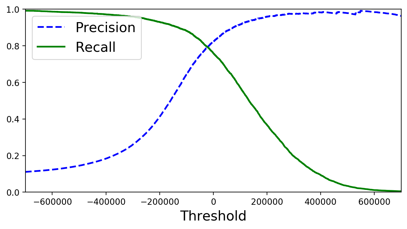
With these scores we can now use the precision_recall_curve() function from
the sklearn.metrics library.
from sklearn.metrics import precision_recall_curve
precisions, recalls, thresholds = precision_recall_curve(y_train_5, y_scores)

def plot_precision_recall_vs_threshold(precisions, recalls, thresholds):
    plt.plot(thresholds, precisions[:-1], "b--", label="Precision", linewidth=2)
    plt.plot(thresholds, recalls[:-1], "g-", label="Recall", linewidth=2)
    plt.xlabel("Threshold", fontsize=16)
    plt.legend(loc="upper left", fontsize=16)
    plt.ylim([0, 1])

plt.figure(figsize=(8, 4))
plot_precision_recall_vs_threshold(precisions, recalls, thresholds)
plt.xlim([-700000, 700000])
# save_fig("precision_recall_vs_threshold_plot")
plt.show()
(y_train_pred == (y_scores > 0)).all()

y_train_pred_90 = (y_scores > 70000)

print(precision_score(y_train_5, y_train_pred_90))

print(recall_score(y_train_5, y_train_pred_90))
0.896551724137931
0.6378896882494005
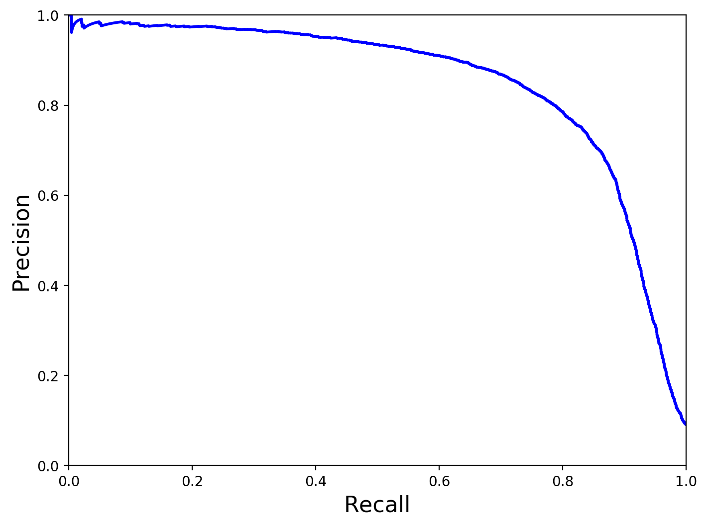
def plot_precision_vs_recall(precisions, recalls):
    plt.plot(recalls, precisions, "b-", linewidth=2)
    plt.xlabel("Recall", fontsize=16)
    plt.ylabel("Precision", fontsize=16)
    plt.axis([0, 1, 0, 1])

plt.figure(figsize=(8, 6))
plot_precision_vs_recall(precisions, recalls)
# save_fig("precision_vs_recall_plot")
plt.show()
25.1.5. ROC curves
from sklearn.metrics import roc_curve
fpr, tpr, thresholds = roc_curve(y_train_5, y_scores)

def plot_roc_curve(fpr, tpr, label=None):
    plt.plot(fpr, tpr, linewidth=2, label=label)
    plt.plot([0, 1], [0, 1], 'k--')
    plt.axis([0, 1, 0, 1])
    plt.xlabel('False Positive Rate', fontsize=16)
    plt.ylabel('True Positive Rate', fontsize=16)

plt.figure(figsize=(8, 6))
plot_roc_curve(fpr, tpr)
# save_fig("roc_curve_plot")
plt.show()
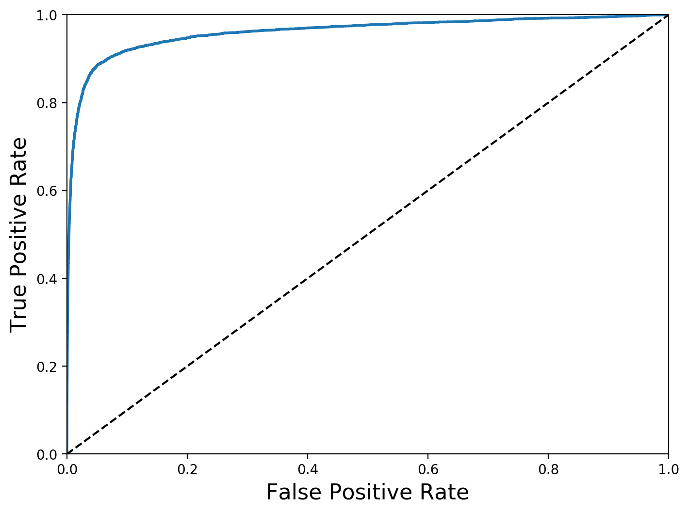
from sklearn.metrics import roc_auc_score
print(roc_auc_score(y_train_5, y_scores))
0.9608926315517949
Note
We set n_estimators=10 to avoid a warning about the fact that its default value will be set to 100 in Scikit-Learn 0.22.
from sklearn.ensemble import RandomForestClassifier
forest_clf = RandomForestClassifier(n_estimators=10, random_state=42)
y_probas_forest = cross_val_predict(forest_clf, X_train, y_train_5, cv=3,
                                    method="predict_proba")

y_scores_forest = y_probas_forest[:, 1] # score = proba of positive class
fpr_forest, tpr_forest, thresholds_forest = roc_curve(y_train_5,y_scores_forest)

plt.figure(figsize=(8, 6))
plt.plot(fpr, tpr, "b:", linewidth=2, label="SGD")
plot_roc_curve(fpr_forest, tpr_forest, "Random Forest")
plt.legend(loc="lower right", fontsize=16)
# save_fig("roc_curve_comparison_plot")
plt.show()
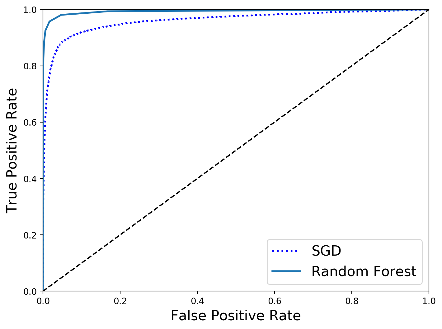
print(roc_auc_score(y_train_5, y_scores_forest))
0.9932680166070984
y_train_pred_forest = cross_val_predict(forest_clf, X_train, y_train_5, cv=3)
precision_score(y_train_5, y_train_pred_forest)

print(recall_score(y_train_5, y_train_pred_forest))
0.8271536616860358
25.2. Key Concepts and Summary
Note
Machine learning
The basic
Some central
25.3. Self-Check Questions
Todo
Why is regression analysis machine learning. What type of machine learning is it?
- Geron2019
Geron, Aurelien (2019), Hands-On Machine Learning with Scikit-Learn, Keras & Tensorflow, O’Reilly, 2nd edition.