16. Random Numbers¶

In this chapter we introduce how to generate random numbers from various distributions in Python. The core library we will be using is the numpy library which contains a powerful random number generator. We will then draw random numbers from different distributions and graph these numbers using histograms in order to check the shape of the distribution that these numbers follow.

16.1. Drawing a Random Number¶

import numpy as np
import matplotlib.pyplot as plt
import math
from scipy import stats as st
import time  # Imports system time module to time your script

plt.close('all')  # close all open figures
tic = time.time()

Let us start with a simple example. Draw a random number that is between zero and one.

myNumber = np.random.uniform(0,1)
print('My first random number in [0,1] is {}'.format(myNumber))

My first random number in [0,1] is 0.8602692305307852

If you run this again you will get a different random number.

myNumber = np.random.uniform(0,1)
print('My second random number in [0,1] is {}'.format(myNumber))

My second random number in [0,1] is 0.42116143252571125

Sometimes it is useful to make sure that the random number sequence that you draw at each run is identical. What you can now do is to set the random number generator on your computer to a specific starting value, or seed. On each run, the same sequence of random numbers is now generated.

np.random.seed(123456789)
myNumber = np.random.uniform(0,1)
print('My first random number in [0,1] is {}'.format(myNumber))

My first random number in [0,1] is 0.532833024789759

Now we reset the seed to the same value again and draw the second random number. You see, this time, it’s identical because it is the first number in a restarted sequence of random numbers.

np.random.seed(123456789)
myNumber = np.random.uniform(0,1)
print('My second random number in [0,1] is {}'.format(myNumber))

My second random number in [0,1] is 0.532833024789759

If you now draw yet another random number without re-setting the seed, you will get a different random number again.

myNumber = np.random.uniform(0,1)
print('My third random number in [0,1] is {}'.format(myNumber))

My third random number in [0,1] is 0.5341366008904166

16.2. Uniformly Distributed Random Numbers¶

You can also draw multiple numbers at the same time without running a loop. In the next example we draw a sequence of 10,000 random numbers from the [0,1] interval.

np.random.seed(123456789)

# Uniform distributed random numbers
u = np.random.uniform(0,1,(10000,))

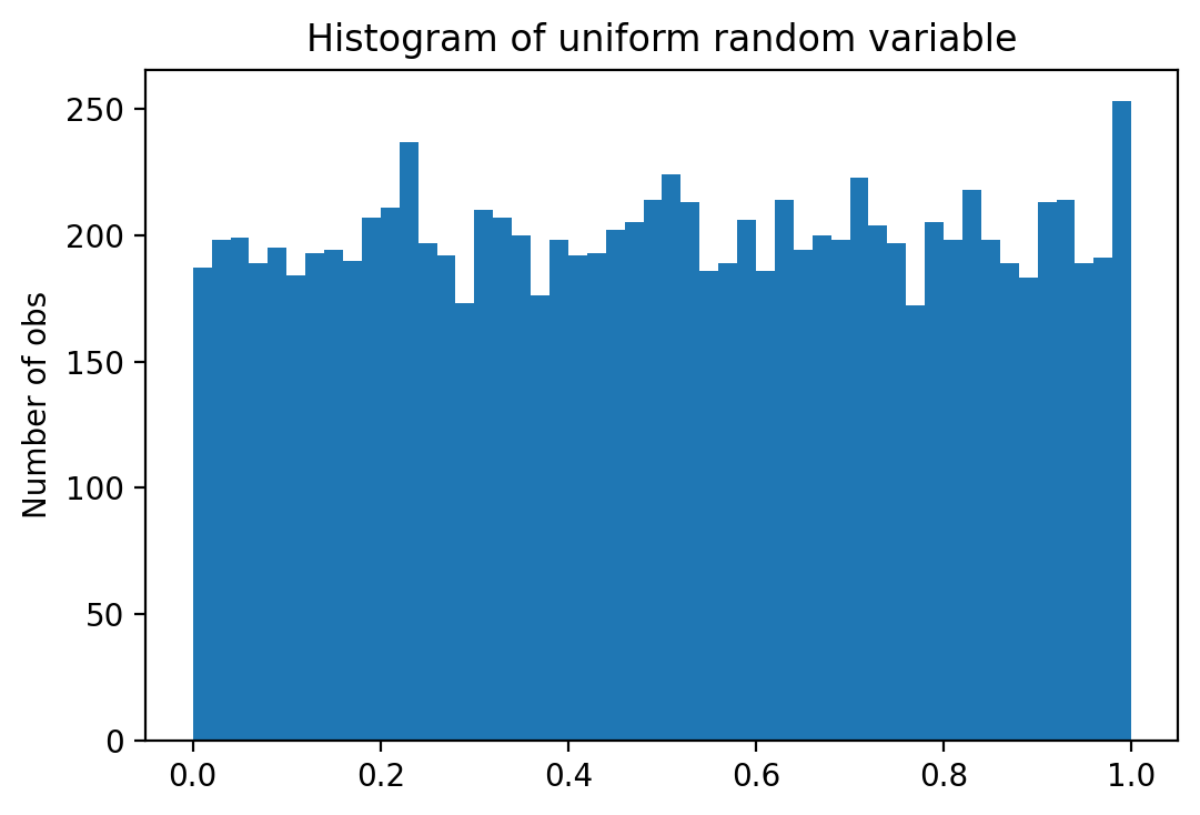
We next make a histogram of these numbers to see the shape of the distribution where they come from. I set the number of bars in the histogram to 30 in order to get a nice picture.

N = 50

fig, ax = plt.subplots()
prob, bins, patches = ax.hist(u, bins=N, align='mid' )
ax.set_ylabel('Number of obs')
ax.set_title('Histogram of uniform random variable')
plt.show()

16.3. Normally distributed random numbers¶

The density function of a normal distribution is:

\[f(x) = \frac{1}{\sigma \times \sqrt{2 \times \pi}} \times e^{-\frac{(x-\mu)^2}{2\times \sigma^2}}\]

where \(\mu\) and \(\sigma\) are the mean and standard deviation the normal distribution.

A standard normal distribution has a mean of zero and a standard deviation of one so that the density function simplifies to

\[f(x) = \frac{1}{\sqrt{2 \times \pi}} \times e^{-\frac{x^2}{2}}\]

def f_phi(x):
    # density function of standard normal
    s = np.exp(-(x**2/2))/np.sqrt(2*np.pi)
    return s

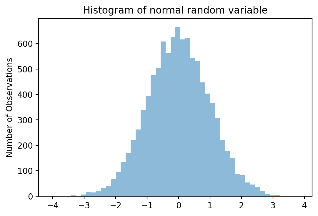
# Draws 10,000 standard normally distributed random numbers
z = np.random.normal(0,1,(10000,))

Then plot it.

fig, ax = plt.subplots()
prob, bins, patches = ax.hist(z, bins=N, align='mid', alpha=0.5)
ax.set_ylabel('Number of Observations')
ax.set_title('Histogram of normal random variable')
#
plt.show()

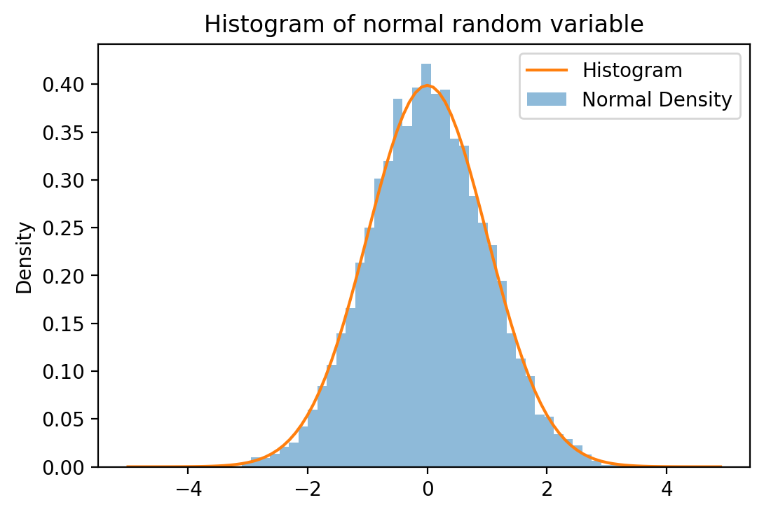
_images/Slides_Random_Normal_Random_1.png

If you want to see the density function used the keyword density. You can then also compare your simulation density with the theoretical density of the Standard Normal distribution.

fig, ax = plt.subplots()
prob, bins, patches = ax.hist(z, bins=N, density=1, align='mid', alpha=0.5)
ax.set_ylabel('Density')
ax.set_title('Histogram of normal random variable')

# Plot the N(0,1) density function into the histogram
x = np.arange(-5,5,0.1)
ax.plot(x, f_phi(x))

ax.legend(['Histogram','Normal Density'], loc='best')
#
plt.show()

_images/Slides_Random_Normal_Random_Density_1.png

Now back to the regular normal distribution with mean mu and standard deviation sigma. Here is the density function in Python with the mean and standard deviation as additional inputs. I also programmed default values for these, so if the user does not specify mean and variance, the function is going to be the standard normal distribution by default.

def f_normalDensity(x, mu=0, sigma=1):
    # density function of standard normal
    s = np.exp(-((x - mu)**2/(2*sigma**2)))/(sigma * np.sqrt(2*np.pi))
    return s

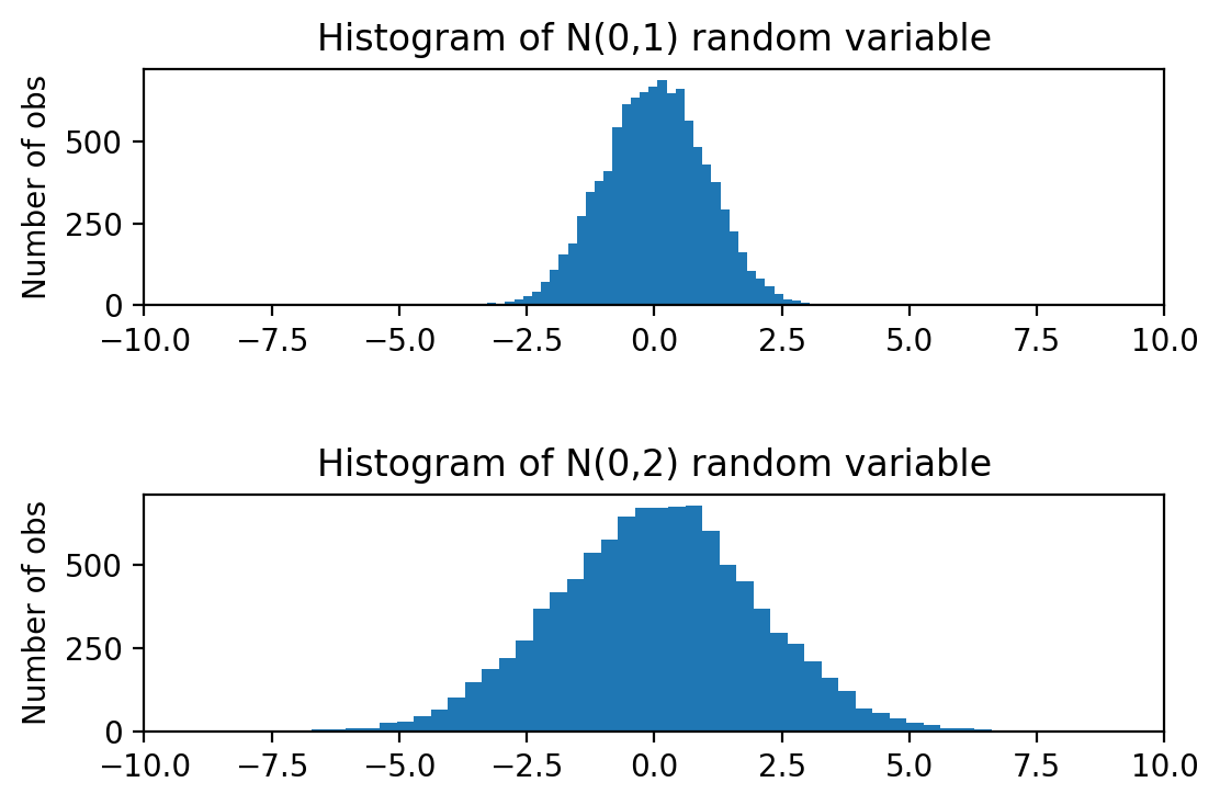
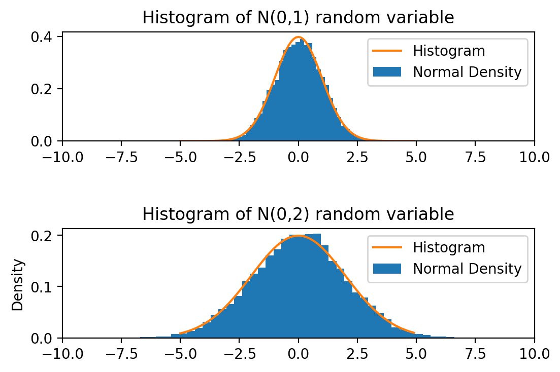
Here is another example of two normally distributed random variables. The first random variable has a smaller standard deviation than the second. Let us see how the distribution of these two compare.

z1 = np.random.normal(0,1,(10000,))
z2 = np.random.normal(0,2,(10000,))

Now plot it.

fig, ax = plt.subplots(2,1)
fig.subplots_adjust(hspace=0.8)
#
prob, bins, patches = ax[0].hist(z1, bins=N, align='mid' )
ax[0].set_ylabel('Number of obs')
ax[0].set_title('Histogram of N(0,1) random variable')
ax[0].set_xlim([-10, 10])
#
prob, bins, patches = ax[1].hist(z2, bins=N, align='mid' )
ax[1].set_ylabel('Number of obs')
ax[1].set_title('Histogram of N(0,2) random variable')
ax[1].set_xlim([-10, 10])

plt.show()

If you want to compare the distribution to the density function again, you can accomplish this by specifying the density option in the hist() method. This makes sure that the area under the curve sums up to one.

fig, ax = plt.subplots(2,1)
fig.subplots_adjust(hspace=0.8)
#
prob, bins, patches = ax[0].hist(z1, density=1, bins=N, align='mid' )
ax[1].set_ylabel('Density')
ax[0].set_title('Histogram of N(0,1) random variable')
ax[0].set_xlim([-10, 10])

# Plot the N(0,1) density function into the histogram
xv = np.arange(-5,5,0.1)
ax[0].plot(xv, f_normalDensity(xv, 0, 1))
ax[0].legend(['Histogram','Normal Density'], loc='best')

#
prob, bins, patches = ax[1].hist(z2, density=1, bins=N, align='mid' )
ax[1].set_ylabel('Density')
ax[1].set_title('Histogram of N(0,2) random variable')
ax[1].set_xlim([-10, 10])
#
ax[1].plot(xv, f_normalDensity(xv, 0, 2))
ax[1].legend(['Histogram','Normal Density'], loc='best')
plt.show()

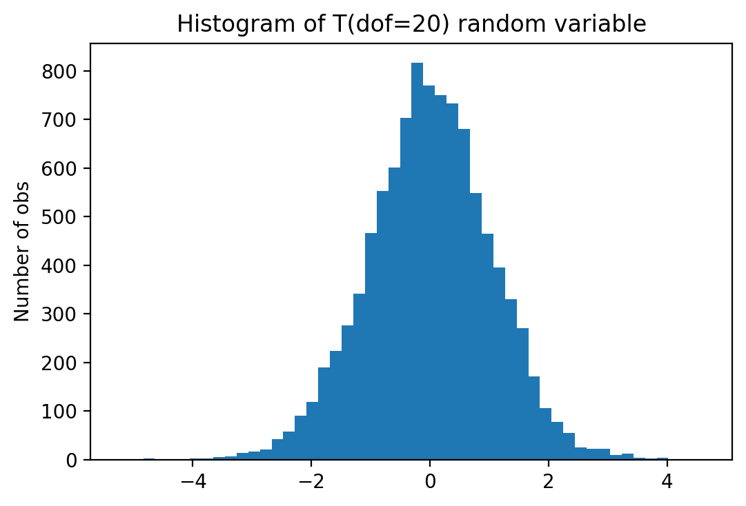
16.4. T-Distributed Random Variable¶

dof = 29
xv = np.random.standard_t(dof, 5)
print(xv)

[ 1.39223765 -0.52924457 -0.82809716 -0.39349782 -1.98709951]

We can also code the t-distribution as a combination of a normal and \(\chi^2\) distribution.

\[ \begin{align}\begin{aligned}X \sim N(0,1)\\Y \sim \chi^2_v\\T = \frac{X}{\sqrt(Y/v)}\end{aligned}\end{align} \]

where \(v\) are the degrees of freedom. The \(\chi^2\) distribution itself can be expressed as a gamma distribution

\[\chi^2_v = \Gamma(1/2, v/2),\]

with \(v\) degrees of freedom.

def student_tvariate(df): # df is the number of degrees of freedom
    if df < 2 or int(df) != df:
        raise ValueError('student_tvariate: df must be a integer > 1')
    x = np.random.normal(0, 1)
    y = np.random.gamma(df/2.0, 2)
    return x / (np.sqrt(y/df))

t = np.zeros((10000),float)
for i in range(10000):
    t[i] = student_tvariate(20)

And the plotting routine is:

fig, ax = plt.subplots()
#
prob, bins, patches = ax.hist(t, bins=N, align='mid' )
ax.set_ylabel('Number of obs')
ax.set_title('Histogram of T(dof=20) random variable')
#
plt.show()

16.5. Drawing Random Integer Values¶

If you want to draw integer numbers at random you can use the np.random.randint() method. If we would like to draw random integer numbers that are either {1,2,3,4} we need to specify np.random.randint(1,5). Note the half open interval definition again that is consistently used across the numpy library.

Note

Alternatively you can use the random library. But be careful, the random library defines random.randint() as closed intervals. The example above using the random library would use random.randint(1,4).

In the following I will always use the random number generator from the numpy library.

import numpy as np

integerList = np.random.randint(1, 5, 10)
print(integerList)

[2 2 3 3 4 4 2 3 1 2]

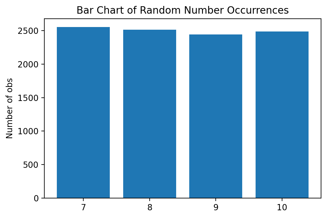
Similarly, if you would like to draw five random integer numbers between 7 and 10 you would specify:

integerList = np.random.randint(7, 11, 5)
print(integerList)

[10  9  9  7  8]

We can again draw 10,000 values and plot them into a bar-chart.

integerList = np.random.randint(7, 11, 10000)

We next count the number of occurrences of each integer value.

xv = np.bincount(integerList)
print(xv)

[   0    0    0    0    0    0    0 2553 2515 2444 2488]

And now we plot the bar-chart with the absolute frequency of each one of the numbers from 7 to 10.

fig, ax = plt.subplots()
ax.bar(7 + np.arange(4), xv[7:11], align='center')
ax.set_xticks(7. + np.arange(4))
ax.set_ylabel('Number of obs')
ax.set_title('Bar Chart of Random Number Occurrences')
plt.show()

16.6. Generating actions based on probabilities¶

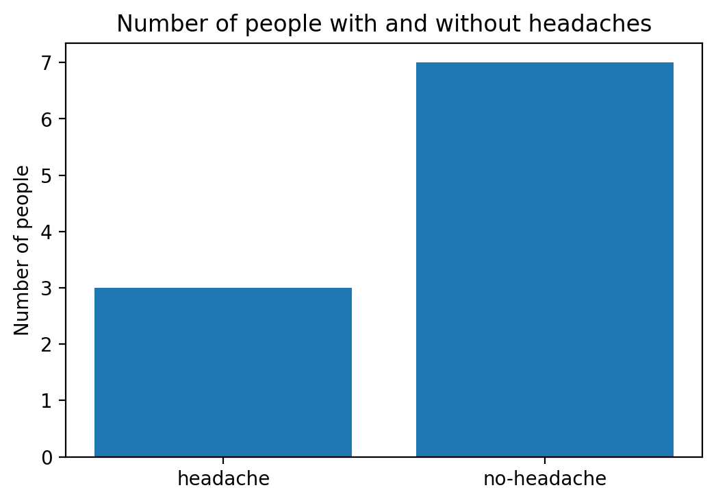
In simulations, statistical applications, or computer games it is often necessary to generate actions based on a certain probability.

For instance, a person wake up in the morning and has a 20 percent chance of having a headache. Simulate 10 people based on this given probability and check how many of them have a headache. We know that theoretically we would expect out of the 10 people, 2 (on average) should wake up with headaches. But of course, waking up with a headache is a probabilistic event, so that it could be that out of the 10 people nobody has a headache, one person has a headache and so on. All of these outcomes are possible but some are more likely than other given the 20 percent probability that we have been given.

In any case, let’s simulate the 10 people. Since we only track whether they have headaches or not (and nothing else), I will not use OOP for this. OOP with a more complete simulation follows in the next section. I will simply collect the information about headaches in a list.

import numpy as np
import matplotlib.pyplot as plt

headacheList  = []

# We now generate 10 "people"
for i in range(10):
    if np.random.rand() <=0.2:
        # Person has headache
        headacheList.append('yes')
    else:
        # Person does not have headache
        headacheList.append('no')

We next plot a bar chart with the absolute frequencies.

# Frequency table
absFreqv = np.array([headacheList.count('yes'), headacheList.count('no')])
labelList = ['headache', 'no-headache']

fig, ax = plt.subplots()
ax.bar(labelList, absFreqv, align='center')
ax.set_ylabel('Number of people')
ax.set_title('Number of people with and without headaches')
plt.show()

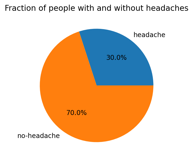
_images/Slides_Random_Bar-Chart-Headache_1.png

And finally a pie chart with the relative frequencies:

# Calculate relative frequencies
relFeqv = absFreqv/np.sum(absFreqv)

fig, ax = plt.subplots()
ax.pie(relFeqv , labels=labelList, autopct='%.1f%%')
ax.set_title('Fraction of people with and without headaches')
plt.show()

_images/Slides_Random_Pie-Chart-Headache_1.png

Note

We have essentially used draws from the uniform distribution as np.random.rand() draws numbers between [0,1] with equal probability i.e., from a uniform distribution. You could also have used np.random.uniform(0,1) to accomplish the same type of random draw.

The same method words for more complicated probability events. Let us say that you have a change of 10 percent of having a headache, a 30 percent chance of having a backache, and a residual 60 percent chance of having no pain at all. You can simulate this easily using the uniform distribution again. Draw the random number using np.random.rand() and

if it is less than 0.1 (happens with a 10 percent chance) you have the headache,

if it is between 0.1 and 0.4 (happens with a 30 percent chance) you have a backache, and

if it is larger than 0.4 (happens with a 60 percent chance) you have no pain.

Here is the implementation:

import numpy as np
import matplotlib.pyplot as plt

painList  = []

# We now generate 10 "people"
for i in range(10):
    randNr = np.random.rand()
    if randNr <=0.1:
        # Person has headache with 10% chance
        painList.append('headache')
    elif randNr >0.1 and randNr <= 0.4:
        # Person has backache with 30% chance
        painList.append('backache')
    else:
        # Person does not have pain with 60%
        painList.append('no-ache')

print(painList)

['no-ache', 'backache', 'no-ache', 'no-ache', 'no-ache', 'headache',
'no-ache', 'no-ache', 'no-ache', 'headache']

You can do the frequency count and graphs as an exercise.

16.7. Drawing Objects with Random Values¶

In this section we demonstrate how we can combine the concepts from the prior chapter on object oriented programing with generating random numbers. We will generate a number of objects whose attributes (or self. variables) will be drawn randomly from certain distributions. In addition we define methods, that will call on random number generators to do something randomly to our objects.

We start by defining our class and the methods that we can subsequently call on these type of objects. We call it the RandomMan class. Objects generated according to this blueprint are then instantiations of this class which we call RandomMan objects.

# Set random seed
np.random.seed(123456789)

class RandomMan(object):
    """This is a random man object.
    RandomMan has a name, numer of children and income.
    RandomMan can showMan(), earnIncome(),
    buyInsurance() and experience and incomeShock()"""

    def __init__(self, name = 'John Doe'):
        """Initialize the man-object with a
        random nr. of children between 0 and 10 and
        with random income drawn from a log-normal distribution
        and an insurance state of 0."""
        self.name = name
        self.children = np.random.randint(0, 10, 1)
        self.income = np.random.lognormal(np.log(50000), 0.2, 1)
        self.insurance = 0  # 0 no insurance, 1 has insurance

    def showMan(self):
        """Method: showMan() prints out
        the variables stored in the man
        object."""
        print("\n")
        print("Hello, let me introduce myself.")
        print("-------------------------------")
        print("My name is {}".format(self.name))
        if self.children == 1:
            # Get grammar right child/children
            print("I have {:1.0f} child" \
                .format(self.children.item()))
        else:
            print("I have {:1.0f} children" \
                .format(self.children.item()))

        print("My income is ${:6.0f}" \
          .format(self.income.item()))
        if self.insurance == 0:
            print("I have NO insurance")
        else:
            print("I have insurance")

    def earnIncome(self, workTime = 0.0):
        """Make man richer by working."""
        self.income += np.sqrt(1 + workTime)

    def buyInsurance(self):
        """Buy insurance if the man is lucky.
        Lucky is define as a [0, 1] random number
        to be smaller than 0.4. So the guy has
        a 40% chance of being lucky. If she is lucky
        she will buy insurance."""
        if np.random.rand()<0.4:
            # Insurance state flips to 1
            self.insurance = 1
            # Insurance costs $100, so the premium is subtracted
            # from her income
            self.income += -100
        else:
            # Insurance state flips to 0
            self.insurance = 0

    def shockIncome(self):
        """Shocks income randomly with a negative
        value between -5000 and 0."""
        if self.insurance == 0:
            # If she has no insurance, her income
            # is randomly reduced
            self.income += np.random.uniform(-5000, 0, 1)

We next generate 10 randomMan objects.

randomManList = []

print(' --- Create men --- ')
for i in range(10):
    # Here we create the randomMan objects and store them in
    # the list
    randomManList.append(RandomMan())
    randomManList[i].showMan()
print(' --- Done --- ')

 --- Create men ---


Hello, let me introduce myself.
-------------------------------
My name is John Doe
I have 8 children
My income is $ 43714
I have NO insurance


Hello, let me introduce myself.
-------------------------------
My name is John Doe
I have 4 children
My income is $ 54296
I have NO insurance


Hello, let me introduce myself.
-------------------------------
My name is John Doe
I have 3 children
My income is $ 63022
I have NO insurance


Hello, let me introduce myself.
-------------------------------
My name is John Doe
I have 2 children
My income is $ 65839
I have NO insurance


Hello, let me introduce myself.
-------------------------------
My name is John Doe
I have 4 children
My income is $ 57828
I have NO insurance


Hello, let me introduce myself.
-------------------------------
My name is John Doe
I have 1 child
My income is $ 56013
I have NO insurance


Hello, let me introduce myself.
-------------------------------
My name is John Doe
I have 3 children
My income is $ 40094
I have NO insurance


Hello, let me introduce myself.
-------------------------------
My name is John Doe
I have 5 children
My income is $ 44958
I have NO insurance


Hello, let me introduce myself.
-------------------------------
My name is John Doe
I have 9 children
My income is $ 55136
I have NO insurance


Hello, let me introduce myself.
-------------------------------
My name is John Doe
I have 0 children
My income is $ 64535
I have NO insurance
 --- Done ---

Finally we let them live for one round.

print('----------------------')
print(' --- Let man live --- ')
print('----------------------')
for i in range(len(randomManList)):
    # Earn income by working randomly between
    # 0 and 40 hours
    randomManList[i].earnIncome(np.random.uniform(0, 40, 1))
    # Buy insurance, if luck
    randomManList[i].buyInsurance()
    # Experience random income shock if NOT insured
    randomManList[i].shockIncome()
    # Show yourself
    randomManList[i].showMan()

----------------------
 --- Let man live ---
----------------------


Hello, let me introduce myself.
-------------------------------
My name is John Doe
I have 8 children
My income is $ 43619
I have NO insurance


Hello, let me introduce myself.
-------------------------------
My name is John Doe
I have 4 children
My income is $ 54201
I have insurance


Hello, let me introduce myself.
-------------------------------
My name is John Doe
I have 3 children
My income is $ 58692
I have NO insurance


Hello, let me introduce myself.
-------------------------------
My name is John Doe
I have 2 children
My income is $ 62261
I have NO insurance


Hello, let me introduce myself.
-------------------------------
My name is John Doe
I have 4 children
My income is $ 57734
I have NO insurance


Hello, let me introduce myself.
-------------------------------
My name is John Doe
I have 1 child
My income is $ 55919
I have insurance


Hello, let me introduce myself.
-------------------------------
My name is John Doe
I have 3 children
My income is $ 38834
I have NO insurance


Hello, let me introduce myself.
-------------------------------
My name is John Doe
I have 5 children
My income is $ 44865
I have insurance


Hello, let me introduce myself.
-------------------------------
My name is John Doe
I have 9 children
My income is $ 50320
I have NO insurance


Hello, let me introduce myself.
-------------------------------
My name is John Doe
I have 0 children
My income is $ 64440
I have insurance

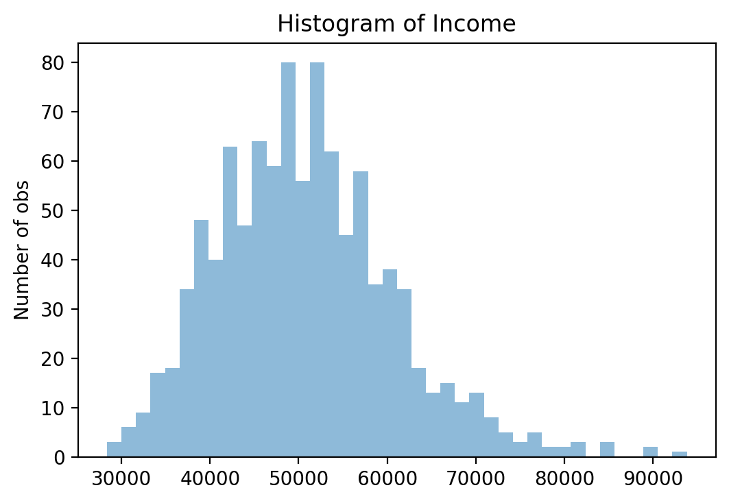
Now let’s blow it up and generate 1,000 random people.

print(' --- Create men --- ')
randomManList = []
N = 1000

for i in range(N):
    # Here we create the randomMan objects and store them in
    # the list
    randomManList.append(RandomMan())

print(' --- Done --- ')

--- Create men ---
--- Done ---

Let’s check the distribution of their income. We know it should look like a normal distribution. Let us first extract the income information and store it into a numpy array (or vector).

incomev = np.zeros(N)

for i in range(N):
    incomev[i] = randomManList[i].income

print('Mean income = {}'.format(incomev.mean()))

Mean income = 50745.14039661928

fig, ax = plt.subplots()
prob, bins, patches = ax.hist(incomev, bins=40, align='mid', alpha=0.5)
ax.set_ylabel('Number of obs')
ax.set_title('Histogram of Income')
plt.show()

_images/Slides_Random_IncomeDistribution_1.png

16.8. Key Concepts and Summary¶

Note

Drawing random numbers
Drawing random numbers from a specific distribution
Writing a simple simulation

16.9. Self-Check Questions¶

Todo

Draw 100 random numbers from a Standard Normal distribution