8. Functions¶

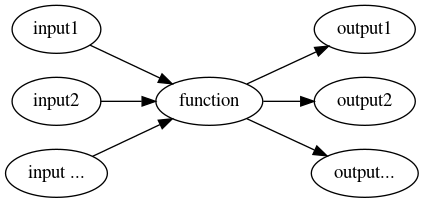
A callable object in Python is an object that can accept some input arguments and possibly return an object or a list of objects. A function is the simplest callable object in Python.

It takes a number of inputs—inputs can be scalars, lists, tuples or objects—and produces a number of outputs—outputs can be scalars, lists, tuples or objects.

digraph {
rankdir="LR";
"input1" -> "function";
"input2" -> "function";
"input ..." -> "function";
"function" -> "output1";
"function" -> "output2";
"function" -> "output...";
}

In Python we use the keyword def to start the function definition code block:

def functionname(input1, input2, ...):
    statement1
    statement2
    obj1 = some calculation
    obj2 = some calculation
    ...
    return obj1, obj2, ...

input1 and input2 are the input arguments. They can be scalars, lists, tuples, objects and even other functions. Variables obj1 and obj2 are output objects that can again be scalars, lists, objects or functions.

The codeblock defined as function can then be called by its name assigned to the output arguments:

out1, out2, ... = functionname(input1, input2, ...)

8.1. A Simple Demonstration Example¶

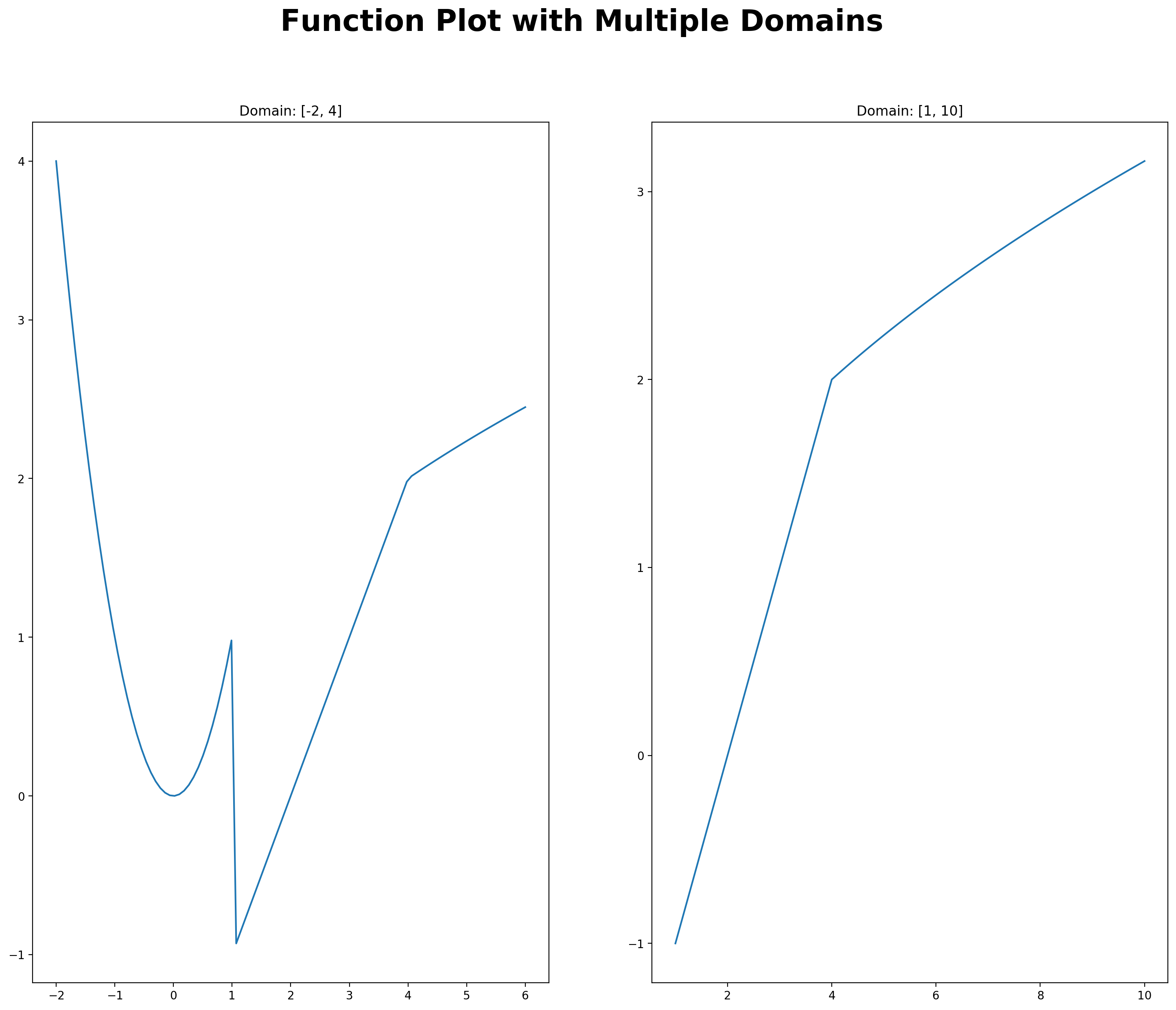
Let’s start with a simple example to demonstrate how powerful functional programming can be. The task is to plot the composite function

f(x) = \begin{cases} x^2 & x < 1 \\ x - 2 & 1 \leq x < 4 \\ \sqrt{x} & 4 \leq x \end{cases}

for two separate domains: \(x\in[-4, 2]\) and \(x\in[1, 10]\).

When plotting a function we typically want to build a table with \(x\) values and the corresponding function values \(y = f(x)\).

\(x\) values	Function Values: \(y=f(x)\)
\(x_0=0\)	\(y_0 = f(0)\)
\(x_1=0.5\)	\(y_1 = f(0.5)\)
\(x_2=1\)	\(y_2 = f(1)\)
\(x_3=1.5\)	\(y_3 = f(1.5)\)
etc.	etc.

Each row in this table describes a point in a \(x-y\) coordinate system. In order to plot the function we collect all the \(x\) values in a vector xv and all the functional values in a vector yv. We then call the plot command plt.plot(xv, yv) to generate the figure.

The problem is now that we have to do this 2 times as you can see in the following script. Where I have indicated the code block that gets repeated.

import numpy as np
import matplotlib.pyplot as plt
import math as m

# Creates  a 1 x 2 grid of subplots
num_rows = 1
num_cols = 2
title_size = 26

# Define empty canvas object
fig = plt.figure(figsize=(18, 14))
fig.suptitle("Function Plot with Multiple Domains", \
    fontsize=title_size, fontweight='bold')
plt.subplots_adjust(wspace=0.2, hspace=0.3)

# Domain [-2, 6]
# ---------------------------------------
# Repeat Code Block
# ---------------------------------------
xv = np.linspace(-2, 6, 100)
yv = np.zeros(len(xv))

for i in range(len(yv)):
    x = xv[i]  # current gridpoint
    if x < 1:
        y = x**2
    elif 1 <= x < 4:
        y = x -2
    else:
        y = m.sqrt(x)
    # Now we store the functional value in
    # the yv vector at current position i
    yv[i] = y
# ---------------------------------------

# [1] We then plot the first figure.
ax = plt.subplot2grid((num_rows, num_cols), (0,0))
ax.plot(xv, yv)
ax.set_title('Domain: [-2, 4]')

# Domain [1, 10]
# ---------------------------------------
# Repeat Code Block
# ---------------------------------------
xv = np.linspace(1, 10, 100)
yv = np.zeros(len(xv))

for i in range(len(yv)):
    x = xv[i]  # current gridpoint
    if x < 1:
        y = x**2
    elif 1 <= x < 4:
        y = x -2
    else:
        y = m.sqrt(x)
    # Now we store the functional value in
    # the yv vector at current position i
    yv[i] = y
# ---------------------------------------

# [2] We then plot the second figure.
ax = plt.subplot2grid((num_rows, num_cols), (0,1))
ax.plot(xv, yv)
ax.set_title('Domain: [1, 10]')
#
plt.show()

_images/Slides_Functions_FigCompFct1_1.png

There is a better way to program this using functions. The strategy is to code the repeated code block only once and assign a name to it. Then, whenever the code block needs to be executed it can simply be called by its name. This will make the script shorter and it will also be easier to maintain.

We use the def keyword to define the function. We will call our function myFunc. The function needs to be on top of your script so that the code block will be named before you call it by its name.

import numpy as np
import matplotlib.pyplot as plt
import math as m

def myFunc(low, high):
    # The function needs two inputs, the lower and
    # upper bound of the function domain!
    # -------------------------------------------
    # Repeat Code Block is now only defined once!
    # -------------------------------------------
    xv = np.linspace(low, high, 100)
    yv = np.zeros(len(xv))

    for i in range(len(yv)):
        x = xv[i]  # current gridpoint
        if x < 1:
            y = x**2
        elif 1 <= x < 4:
            y = x -2
        else:
            y = m.sqrt(x)
        # Now we store the functional value in
        # the yv vector at current position i
        yv[i] = y
    # -------------------------------------------
    # In the return statement we declare the output of the function.
    # In this example the output is composed of 2 vectors: xv and yv.
    # When you call this function, make sure you call it with two
    # vectors as output such as: vec1, vec2 = myFunc(low, high)
    # The results will then be stored in the two
    # vectors vec1 anc vec2
    return xv, yv

# Creates  a 1 x 2 grid of subplots
num_rows = 1
num_cols = 2
title_size = 26

# Define empty canvas object
fig = plt.figure(figsize=(18, 14))
fig.suptitle("Function Plot with Multiple Domains", \
    fontsize=title_size, fontweight='bold')
plt.subplots_adjust(wspace=0.2, hspace=0.3)

# Domain [-2, 6]
x1v, y1v = myFunc(-2, 6)
# Domain [1, 10]
x2v, y2v = myFunc(1, 10)

# [1] We then plot the first figure.
ax = plt.subplot2grid((num_rows, num_cols), (0,0))
ax.plot(x1v, y1v)
ax.set_title('Domain: [-2, 4]')
# [2] We then plot the second figure.
ax = plt.subplot2grid((num_rows, num_cols), (0,1))
ax.plot(x2v, y2v)
ax.set_title('Domain: [1, 10]')
#
plt.show()

_images/Slides_Functions_FigCompFct2_1.png

As you can see this second script is much shorter than the first. It is also easier to maintain and fix. If you have to add more domain plots you simply call the function more times which is just one extra line of code as opposed to copying the entire code block again as in the first version of the script.

Second, if you find that your function definition contains a mistake, you only have to fix it once in the function definition and all the subsequent function calls and corresponding plots will automatically be updated to the latest and correct version. In the first version of the code you would have to make changes twice which is more work and more error prone.

8.2. Simple User Defined Function in Separate File¶

In Python we can write the following to define a simple function. We start with two simple function definitions and save them in a file called myFunctions.py

import numpy as np
import matplotlib.pyplot as plt
import math as m
from scipy import stats as st
# Imports system time module to time your script
import time
# Needed for re-loading user defined function-modules
import imp

plt.close('all')  # close all open figures

We next define our own functions and save them as myFunctions.py

# File 1: myFunctions.py
def hw1(r1, r2):
    s = m.sin(r1 + r2)
    return s

def hw2(r1, r2):
    s = m.sin(r1 + r2)
    print("Hello, World! sin({0:4.2f}+{1:4.2f}) = {2:4.2f}".format(r1, r2, s))

In a separate Python script we can now import this previous file containing our functions with the import command. We save this new Python script as Lecture_Functions/myFunctions.py

# NOTE: If the myFunctions.py is stored in the same location than the script
# file you are currently running, then you do not need these complicated import
# statements on the next two lines.

# File 2 stored in: Lecture_Functions/myFunctions.py
import sys
sys.path.insert(0,'/home/jjung/Dropbox/Towson/teaching/2_ComputationalEconomics/LecturesNew/source/Lecture_Functions')

# Skip the above and start here if your function file is stored in the same
# location as your script file.

import myFunctions as mfunc
# This next line makes sure that if you
# edited the file myfunctions.py -> the
# import is updated!
imp.reload(mfunc)

# Now we call these functions with function arguments
print(mfunc.hw1(2.6, 4.0))
mfunc.hw2(2.5,5.6)

0.31154136351337786
Hello, World! sin(2.5+5.6)=0.96989

8.3. Advanced Graphing using Loops and Functions¶

8.3.1. Graphing Functions with two Input Arguments z = f(x,y)¶

We next want to plot a function with two input variables:

\[f(x,y) = sin(x \times y).\]

We first define an input grid for values of \(x\) and store the grid in vector xv, followed by an input grid for values of \(y\) which is stored in vector yv.

from mpl_toolkits.mplot3d import Axes3D

xv = np.arange(1, 11, 1)
yv = np.arange(1, 11, 1)

# Meshgrid spans a grid-field over the 2 dimensions
X, Y = np.meshgrid(xv, xv)

# X and Y are both matrices now
xn, yn = X.shape

# We next need to evaluate the function
# repeatedly over the entire grid-field

# Define matrix size n x n with zero entries
f = np.zeros((xn, yn),float)
for i in range(xn):
    for j in range(yn):
        #print(i,j)
        # Here you want to use matrix X
        # and not the gridvector xv
        f[i,j] = np.sin(X[i,j]*Y[i,j])

fig = plt.figure(figsize=(14,16))
ax = Axes3D(fig)
ax.plot_wireframe(X, Y, f, rstride=2, cstride=2)
ax.set_xlabel('x')
ax.set_ylabel('y')
ax.set_zlabel('f(x,y)')
ax.set_title('sin(x,y)')
plt.show()

_images/Slides_Functions_Fig3DPlot_1.png

8.3.2. Same Thing but Different Function¶

This time we define the function first using the def command:

\[g = f(x, y)=(1 + y * 2) ^ {(-x / y)} * (1 + y * 1) ^ {(x / y)}\]

We then span a grid over x and y and evaluate the function g at each combination of (x,y) using the expand.grid command.

The grid space between (x,y) is created using the meshgrid command. The function g is then evaluated at every point (x,y) over the grid. The ax.plot_wireframe command produces the picture.

# Define function
def g(x, y):
    res = (1 + y * 2) ** (-x / y) * (1 + y * 1) ** (x / y)
    return res

xv = np.linspace(0.01, 1, 20)
yv = np.linspace(0.01, 1, 20)
X, Y = np.meshgrid(xv, yv)

xn, yn = X.shape

f = np.zeros((xn,xn),float)   # Define matrix size nxn with zero entries
for i in range(xn):
    for j in range(yn):
        f[i,j] = g(X[i,j], Y[i,j])

fig = plt.figure(figsize=(14,16))
ax = Axes3D(fig)
ax.plot_wireframe(X, Y, f, rstride=2, cstride=2)
ax.set_title('sin(x,y)')
ax.set_xlabel('x')
ax.set_ylabel('y')
ax.set_zlabel('f(x,y)')
plt.show()

8.4. Functions with Default Arguments¶

A default argument is an argument that assumes a default value if a value is not provided in the function call for that argument. The following example illustrates default arguments in a simple function with two inputs, a name and a number, that the function then prints in the terminal window.

def f_printInfo(name, age = 35):
    "This prints the passed variable values"
    print('-----------------')
    print("Name: {}".format(name))
    print("Age: {}".format(age))
    print('-----------------')
    return

We next call the function by differently assigning the name and age variables.

f_printInfo(age=50, name="mike")

-----------------
Name: mike
Age: 50
-----------------

f_printInfo(name="mike")

-----------------
Name: mike
Age: 35
-----------------

This next function call is problematic as it reverses the variable order!

f_printInfo(50, "john")

-----------------
Name: 50
Age: john
-----------------

If you want to reverse the order you need to provide the keyword argument

so that the function can assign the values correctly.

f_printInfo(name="mike", age=50)

-----------------
Name: mike
Age: 50
-----------------

And this one throws a syntax error since we are inconsistent with out function call by providing a keyword argument for one of the input variables but not for the other and we reverse the order at the same time. Here the interpreter will not be able to figure out the correct correspondence between inputs and variable assignments and therefore it throws an error.

f_printInfo(name="mike", 50)

  File "<ipython-input-1-95c77d76a7d9>", line 1
    f_printInfo(name="mike", 50)
                            ^
SyntaxError: positional argument follows keyword argument

8.5. Scope of Variables in Functions¶

When we use functions we need to distinguish between variables that are local to functions and that can therefore be readily accessed and manipulated by the functions and variables that are defined outside of a function. These variables usually cannot be manipulated directly from within a function.

def myFun(x):
    x += 1
    print('x in myFun = ', x)

# Call function
x = 10
myFun(5)
print('x outside function = ', x)

x in myFun =  6
x outside function =  10

Now let’s try to access a variable that is defined outside of the function in what is called the global name space as opposed to the local name space inside of the function.

def myFun2(x):
    x += 1
    print('x inside myFun2 = ', x)
    print('y inside myFun2 = ', y)

# Call function
y = 10
myFun2(5)

x inside myFun2 =  6
y inside myFun2 =  10

Here we see that it is still possible to access variable y despite the fact that it is not handed in explicitly.

Warning

This is bad programming style and should be avoided. Always try to be as explicit as possible. If you want to use input argument y in your function, then define it explicitly as input argument.

Let us now try to change the value of variable y inside of the function.

def myFun3(x):
    x += 1
    print('x inside myFun3 = ', x)
    y = 5
    print('y inside myFun3 = ', y)

# Call function
y = 10
myFun3(5)
print('y outside function =', y)

x inside myFun3 =  6
y inside myFun3 =  5
y outside function = 10

Here we use variable y again and define it as a local variable inside the function. However, this change is only valid inside the local name space of the function. Once we are outside the function the value of y is 10 again. So y has now two instances, one in the local name space inside the function and another one in the global name space outside of the function.

Let’s next try to manipulate a variable that is not explicitly handed into the function.

def myFun4(x):
    x += 1
    print('x inside myFun4 = ', x)
    print('y inside myFun4 = ', y)
    y = 1
    print('y inside myFun4 = ', y)

# Call function
y = 10
myFun4(5)
print('y outside function =', y)

x inside myFun4 =  6

---------------------------------------------------------------------------UnboundLocalError
Traceback (most recent call last)<ipython-input-1-897c56e0726e> in
<module>
      8 # Call function
      9 y = 10
---> 10 myFun4(5)
     11 print('y outside function =', y)
<ipython-input-1-897c56e0726e> in myFun4(x)
      2     x += 1
      3     print('x inside myFun4 = ', x)
----> 4     print('y inside myFun4 = ', y)
      5     y = 1
      6     print('y inside myFun4 = ', y)
UnboundLocalError: local variable 'y' referenced before assignment

Here we get an error because the interpreter defines y as local variable and the first print statement happens before the local variable y is defined.

We could finally use variable y as a global variable in which case we can change it outside and inside the function.

Warning

Again, this is considered bad programming style as it can very quickly lead to errors that will be difficult to spot.

def myFun5(x):
    global y
    x += 1
    print('x inside myFun5 = ', x)
    print('y inside myFun5 = ', y)
    y += 1
    print('y inside myFun5 = ', y)

# Call function
y = 10
print('y outside function =', y)
myFun5(5)
print('y outside function =', y)

y outside function = 10
x inside myFun5 =  6
y inside myFun5 =  10
y inside myFun5 =  11
y outside function = 11

8.6. Scope of Lists and Arrays in Functions¶

The scoping is a little tricky with lists. Check out the following code:

def myList(inList):
    # This creates a local name that points to the same list.
    # If you change this local name list you actually also
    # change the original list
    localList = inList
    print('inside function: ', localList)
    localList.append('bruno')
    print('inside function: ', localList)
    return localList

Calling this function you may expect that the local list should be different from the list that is handed in from the global namespace. However, the following will happen when you call the function:

queue = ["Steve", "Russell", "Alison", "Liam"]
print('outside: ', queue)
myList(queue)
print('outside: ', queue)

outside:  ['Steve', 'Russell', 'Alison', 'Liam']
inside function:  ['Steve', 'Russell', 'Alison', 'Liam']
inside function:  ['Steve', 'Russell', 'Alison', 'Liam', 'bruno']
outside:  ['Steve', 'Russell', 'Alison', 'Liam', 'bruno']

We see that the local operation on the list has now affected the global list as well. Why is that? It has to do with how Python treats list assignments. When you assign a list to a new name, you do not create a new list object. The new name simply points to the same location in the computer’s memory where the original list is saved. This preserves space. If you now start manipulating the list under its new name, it will translate into changes when calling the same list under its old name (in the global namespace) as well.

In the previous example with numbers we did not have to worry about this. When we assigned a new scalar to a variable name, it immediately generates a new object. Local changes to this separate instance would therefore not affect the variable in the global namespace.

Note

If you want the same behavior when working with lists, you need to deepcopy the list. This will effectively create a new list object inside the function scope. Changes in this new object will not trigger changes in the old list object that resides in the global namespace.

Try this definition:

import copy

def myList2(inList):
    # This creates a new local list object
    localList = copy.deepcopy(inList)
    print('inside function: ', localList)
    localList.append('bruno')
    print('inside function: ', localList)
    return localList

If you call this, we now have a separate list in the global and local namespace.

queue2 = ["Steve", "Russell", "Alison", "Liam"]
print('outside: ', queue2)
myList2(queue2)
print('outside: ', queue2)

outside:  ['Steve', 'Russell', 'Alison', 'Liam']
inside function:  ['Steve', 'Russell', 'Alison', 'Liam']
inside function:  ['Steve', 'Russell', 'Alison', 'Liam', 'bruno']
outside:  ['Steve', 'Russell', 'Alison', 'Liam']

If you deal with numpy arrays you do not have to worry about this. As a new assignment of a numpy array will always generate a new object (just like a number assignment did in the previous section) and not a new pointer to an existing space in memory. Try this:

def myArray(inArray):
    # This creates a local name that is a new object
    localArray = inArray
    print('inside function: ', localArray)
    localArray = np.append(localArray,4)
    print('inside function: ', localArray)
    return localArray

And calling it:

queue = np.array([1,2,3])
print('outside: ', queue)
myArray(queue)
print('outside: ', queue)

outside:  [1 2 3]
inside function:  [1 2 3]
inside function:  [1 2 3 4]
outside:  [1 2 3]

8.7. Key Concepts and Summary¶

Note

Functions allow you to collect a code block that gets repeated a lot.
Functions take input variables and produce an output variable or variables.
Functions allow you to keep your codes shorter

8.8. Self-Check Questions¶

Todo

Program a function that calculates the standard deviation of the elements of an input vector. Then evaluate the function with this vector \(\vec{x}=[0.4, 0.6,0.9,1.8,4.2,2.9]\)