24. Machine Learning I: Introduction to Machine Learning
This chapter and the next are heavily built on two chapters in [Geron2019] Hands-On Machine Learning with Scikit-Learn, Kera & TensorFlow. You can find a link to the GitHub page of this textbook at Geron GitHub
Machine learning is ubiquitous. Machine learning algorithm guide your daily google searches, determine the way Netflix presents its offerings to you, guide your selections when shopping on sites such as Amazon, translate your spoken words into code that your Phone or any other of the many voice assistants can process further into meaningful services for you, drive Teslas semi-autonomous, or simply recognize your face on a photo you upload onto Facebook. These are just a few of the many many examples where Machine Learning has entered your life, whether you are aware of it or not.

Fig. 24.1 Brief History of Machine Learning
One of the earliest examples of a Machine Learning algorithm that you are familiar with is the Spam Filter. We will be using this example to further explain what machine learning does and how different machine learning algorithms can be classified.
24.1. Different Types of Machine Learning Algorithms
Machine learning algorithms can be classified according to the following criteria:
- Supervised vs. unsupervised vs. reinforcement learning
Are they trained (estimated) with human supervision, without supervision, or do they reinforce actions based on rewards and penalties.
- Online vs. batch learning
Do they learn incrementally as data becomes available or do they require “all of the data” at once
- Instance-based vs. model-based learning
Do they compare new data points to known data points or do they detect patterns building a predictive model (based on parameters)
Let’s discuss this classification in some more detail. In supervised learning, the training set (i.e., data) you feed to the algorithm includes the desired outcome or solution, called label (i.e., the dependent or outcome variable). In other words, if you know what your outcome variable is, i.e., what it measures, then we say it has a label because you are able to classify the outcome variable according to some criteria.
If, on the other hand, you do not even know what exactly your outcome variable is, i.e., it is missing a label that would allow a quick classification of this variable, then we are talking about so called Unsupervised learning which deals with unlabeled data. In this instance we are usually trying to find some patterns in the outcome variable that we can then use for a possible interpretation of what the outcome variable actually measures.
Fig. 24.2 summarizes the different types of machine learning according to our first classification above where we distinguished between
Supervised Learning,
Unsupervised Learning, and
Reinforcement Learning.

Fig. 24.2 Classification of ML algorithms.
Table 24.1 contrasts the language we use in Econometrics with the language commonly used in Machine Learning.
Item |
Econometrics |
Machine Learning2011 |
|---|---|---|
Data |
Data/Obs. |
Training data/set |
y |
Dependent var |
Label |
x or X |
Independent var |
Feature/predictor |
Estimation |
Training an algorithm or model |
24.2. A First Regression Model Example
24.2.1. Downloading the Data
We again start by first importing some libraries.
# https://github.com/ageron/handson-ml/
import numpy as np
import pandas as pd
import os
import tarfile
from six.moves import urllib
We first need to download the data from GitHub:
DOWNLOAD_ROOT = "https://raw.githubusercontent.com/ageron/handson-ml/master/"
HOUSING_URL = DOWNLOAD_ROOT + "datasets/housing/housing.tgz"

def fetch_housing_data(housing_url=HOUSING_URL):
    tgz_path = os.path.join("housing.tgz")
    urllib.request.urlretrieve(housing_url, tgz_path)
    housing_tgz = tarfile.open(tgz_path)
    housing_tgz.extractall()
    housing_tgz.close()

fetch_housing_data()
Once that is done, we store the
data on our local drive. You want to avoid downloading the data each time you
run the script file. So download it once, store it and then comment the
download section of your code out and just read the data from your local drive
using the pd.read_csv() function from the numpy library.
We then can use a few commands to look at our data which is organized or stored in a
Pandas DataFrame object.
housing = pd.read_csv("Lecture_MachineLearning_1/housing.csv")

print(housing.head())
   longitude  latitude  housing_median_age  total_rooms
total_bedrooms  \
0    -122.23     37.88                41.0        880.0
129.0
1    -122.22     37.86                21.0       7099.0
1106.0
2    -122.24     37.85                52.0       1467.0
190.0
3    -122.25     37.85                52.0       1274.0
235.0
4    -122.25     37.85                52.0       1627.0
280.0

   population  households  median_income  median_house_value
ocean_proximity
0       322.0       126.0         8.3252            452600.0
NEAR BAY
1      2401.0      1138.0         8.3014            358500.0
NEAR BAY
2       496.0       177.0         7.2574            352100.0
NEAR BAY
3       558.0       219.0         5.6431            341300.0
NEAR BAY
4       565.0       259.0         3.8462            342200.0
NEAR BAY
We can get a quick summary of our data using the .info() function on the
dataframe.
print(housing.info())
<class 'pandas.core.frame.DataFrame'>
RangeIndex: 20640 entries, 0 to 20639
Data columns (total 10 columns):
 #   Column              Non-Null Count  Dtype
---  ------              --------------  -----
 0   longitude           20640 non-null  float64
 1   latitude            20640 non-null  float64
 2   housing_median_age  20640 non-null  float64
 3   total_rooms         20640 non-null  float64
 4   total_bedrooms      20433 non-null  float64
 5   population          20640 non-null  float64
 6   households          20640 non-null  float64
 7   median_income       20640 non-null  float64
 8   median_house_value  20640 non-null  float64
 9   ocean_proximity     20640 non-null  object
dtypes: float64(9), object(1)
memory usage: 1.6+ MB
None
24.2.2. Inspecting the Data
We can also get some summary statistic for specific feature variables (in
econometrics we refer to these as independent variables). We can check the
variable ocean_proximity for instance. It is a categorical variable. We
cannot do any numerical statistics with this but we can get a feel for this
variable by counting how many observation by category we have.
print(housing["ocean_proximity"].value_counts())
<1H OCEAN     9136
INLAND        6551
NEAR OCEAN    2658
NEAR BAY      2290
ISLAND           5
Name: ocean_proximity, dtype: int64
Finally, we can use the .describe() dataframe method (or function) to get
certain summary statistics for each data column.
print(housing.describe())
          longitude      latitude  housing_median_age   total_rooms  \
count  20640.000000  20640.000000        20640.000000  20640.000000
mean    -119.569704     35.631861           28.639486   2635.763081
std        2.003532      2.135952           12.585558   2181.615252
min     -124.350000     32.540000            1.000000      2.000000
25%     -121.800000     33.930000           18.000000   1447.750000
50%     -118.490000     34.260000           29.000000   2127.000000
75%     -118.010000     37.710000           37.000000   3148.000000
max     -114.310000     41.950000           52.000000  39320.000000

       total_bedrooms    population    households  median_income  \
count    20433.000000  20640.000000  20640.000000   20640.000000
mean       537.870553   1425.476744    499.539680       3.870671
std        421.385070   1132.462122    382.329753       1.899822
min          1.000000      3.000000      1.000000       0.499900
25%        296.000000    787.000000    280.000000       2.563400
50%        435.000000   1166.000000    409.000000       3.534800
75%        647.000000   1725.000000    605.000000       4.743250
max       6445.000000  35682.000000   6082.000000      15.000100

       median_house_value
count        20640.000000
mean        206855.816909
std         115395.615874
min          14999.000000
25%         119600.000000
50%         179700.000000
75%         264725.000000
max         500001.000000
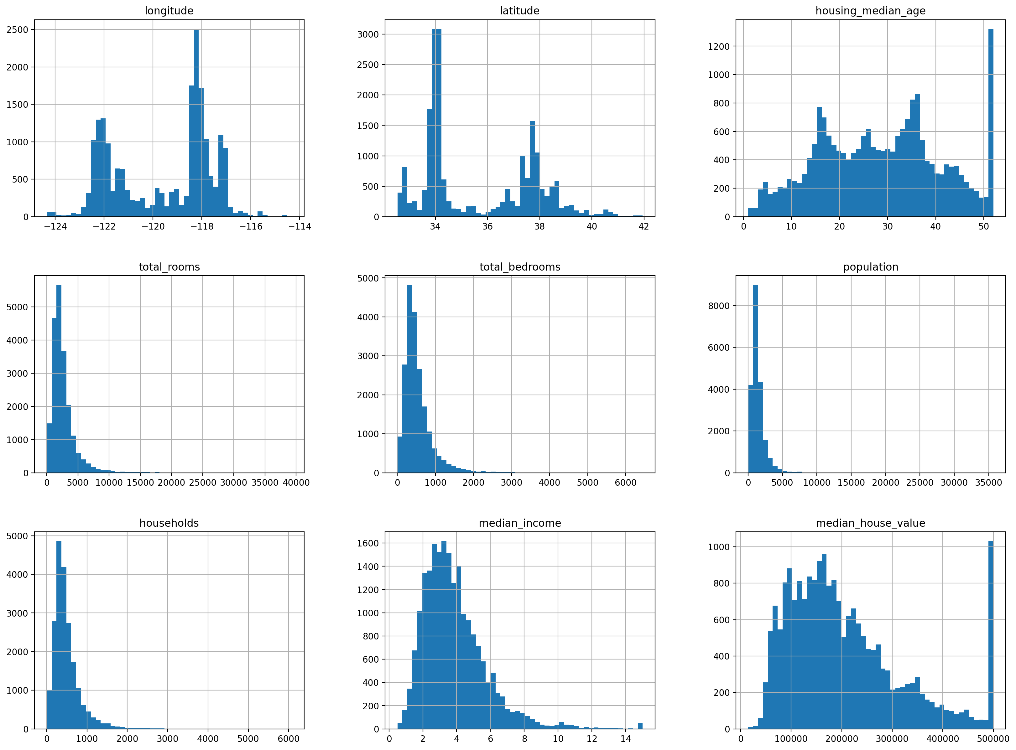
We next start with analyzing our data using graphs and simple statistics.
# %matplotlib inline
import matplotlib.pyplot as plt
housing.hist(bins=50, figsize=(20,15))
# save_fig("attribute_histogram_plots")
plt.show()
24.2.3. Splitting the Data
In machine learning it is important to be able to assess how well your trained model can predict outcome variables (or label variables in the case of supervised machine learning). In order to do this we need to split the sample into a training sample that you use to train (estimate) the model with and into a test sample that you can then use to verify how well your model makes out of sample predictions.
It is important that you randomly split the sample and that both samples maintain the features of the overall sample. For instance if your main sample contains 45 percent men, then you want to split the sample in such a way that the training sample has roughly 45 percent men in it and the test sample has roughly 45 percent men in it.
In order to accomplish this we use the built in command train_test_split
from the sklearn machine learning library. When you call this function you
need to specify how large you want the test sample to be. Below we choose a
split that maintains 80 percent of the observations in the raw data for
the training sample and 20 percent for test sample. We set the random seed by
hand, so that our results become reproducible, i.e., the sample is split in
exactly the same way each time we run the script file.
from sklearn.model_selection import train_test_split

# to make this notebook's output identical at every run
np.random.seed(42)

train_set, test_set = train_test_split(housing, test_size=0.2, random_state=42)
We can now inspect the test sample.
print(test_set.head())
       longitude  latitude  housing_median_age  total_rooms
total_bedrooms  \
20046    -119.01     36.06                25.0       1505.0
NaN
3024     -119.46     35.14                30.0       2943.0
NaN
15663    -122.44     37.80                52.0       3830.0
NaN
20484    -118.72     34.28                17.0       3051.0
NaN
9814     -121.93     36.62                34.0       2351.0
NaN

       population  households  median_income  median_house_value  \
20046      1392.0       359.0         1.6812             47700.0
3024       1565.0       584.0         2.5313             45800.0
15663      1310.0       963.0         3.4801            500001.0
20484      1705.0       495.0         5.7376            218600.0
9814       1063.0       428.0         3.7250            278000.0

      ocean_proximity
20046          INLAND
3024           INLAND
15663        NEAR BAY
20484       <1H OCEAN
9814       NEAR OCEAN
One thing that is important when splitting the data is to maintain the composition of the data in the subsamples, so that subsamples correctly represent the large sample. Let us look at an example.
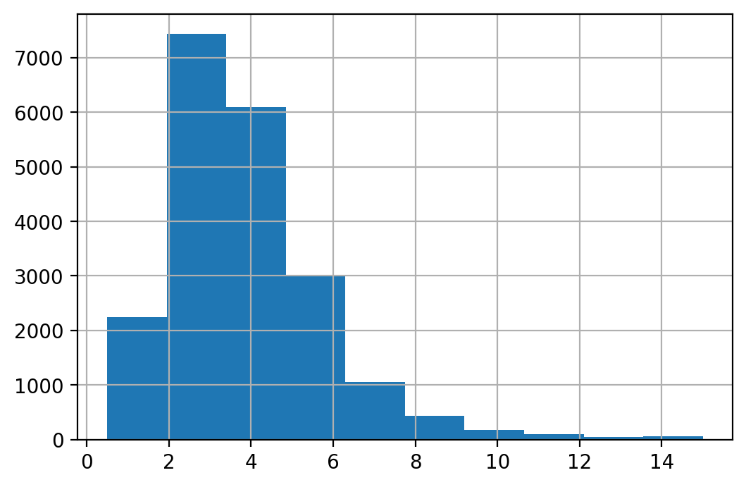
If we analyze income using the histogram plot we have the following distribution of income.
housing["median_income"].hist()
<AxesSubplot:>
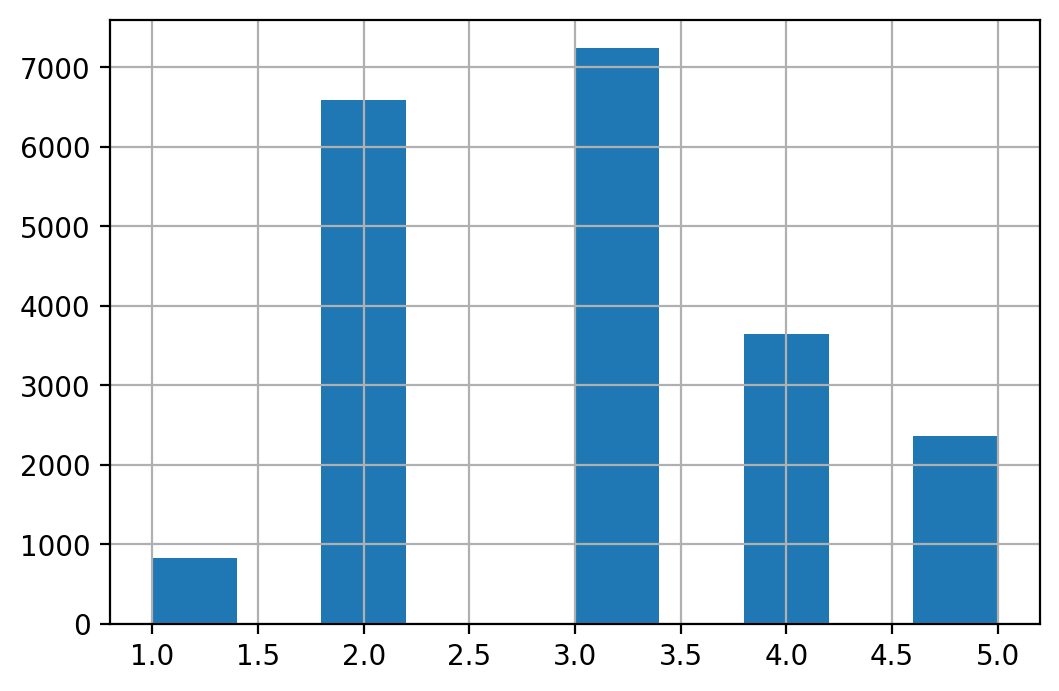
We can also make a categorical variable out of income using the following command.
housing["income_cat"] = pd.cut(housing["median_income"],
                               bins=[0., 1.5, 3.0, 4.5, 6., np.inf],
                               labels=[1, 2, 3, 4, 5])
In order to do that we need to define the bins and assign labels to each bin.
Where label 1 indicates the low income group, label 2 indicates income
between zero and 1.5, etc. We can then plot histograms of this new categorical
variable.
print(housing["income_cat"].value_counts())

housing["income_cat"].hist()
3    7236
2    6581
4    3639
5    2362
1     822
Name: income_cat, dtype: int64
<AxesSubplot:>
When we split the sample into a training set and a test set we need to make
sure that the distribution of the different income groups is maintained in the
subsamples. We want to avoid as situation where we have, let’s say richer
households in the training sample and relatively poorer households in the
testing sample. We can accomplish this with stratified sampling. The built in
command StratifiedShuffleSplit will split the data ensuring that the
distribution is maintained.
from sklearn.model_selection import StratifiedShuffleSplit

split = StratifiedShuffleSplit(n_splits=1, test_size=0.2, random_state=42)
for train_index, test_index in split.split(housing, housing["income_cat"]):
    strat_train_set = housing.loc[train_index]
    strat_test_set = housing.loc[test_index]
We can check this by comparing the histogram we made earlier for the entire data with the histogram for the income variables of the stratified test sample. You see that the proportions of the different income groups are maintained because we split the sample according to the income strata in the above code block.
print(strat_test_set["income_cat"].value_counts() / len(strat_test_set))
3    0.350533
2    0.318798
4    0.176357
5    0.114341
1    0.039971
Name: income_cat, dtype: float64
We can compare it to the income categories of the original data.
print(housing["income_cat"].value_counts() / len(housing))
3    0.350581
2    0.318847
4    0.176308
5    0.114438
1    0.039826
Name: income_cat, dtype: float64
We next do it more systematic across the full data, the stratified test set, and the non-stratified test set. We then plot the proportions of the income groups for each data set. You want the proportions in the test set be very close to the income proportions in the full data.
def income_cat_proportions(data):
    return data["income_cat"].value_counts() / len(data)

train_set, test_set = train_test_split(housing, test_size=0.2, random_state=42)

compare_props = pd.DataFrame({
    "Overall": income_cat_proportions(housing),
    "Stratified": income_cat_proportions(strat_test_set),
    "Random": income_cat_proportions(test_set),
}).sort_index()
compare_props["Rand. %error"] = 100 * compare_props["Random"] / compare_props["Overall"] - 100
compare_props["Strat. %error"] = 100 * compare_props["Stratified"] / compare_props["Overall"] - 100
Now let’s have a look at the different methods and how they compare to the original data.
print(compare_props)
    Overall  Stratified    Random  Rand. %error  Strat. %error
1  0.039826    0.039971  0.040213      0.973236       0.364964
2  0.318847    0.318798  0.324370      1.732260      -0.015195
3  0.350581    0.350533  0.358527      2.266446      -0.013820
4  0.176308    0.176357  0.167393     -5.056334       0.027480
5  0.114438    0.114341  0.109496     -4.318374      -0.084674
Before we move on, we drop the income category variable because we do not use this categorical variable in our “forecasting” model.
for set_ in (strat_train_set, strat_test_set):
    set_.drop("income_cat", axis=1, inplace=True)
24.2.4. Visualize data to gain insight
We next copy the stratified training data set and assign it a shorter name.
housing = strat_train_set.copy()
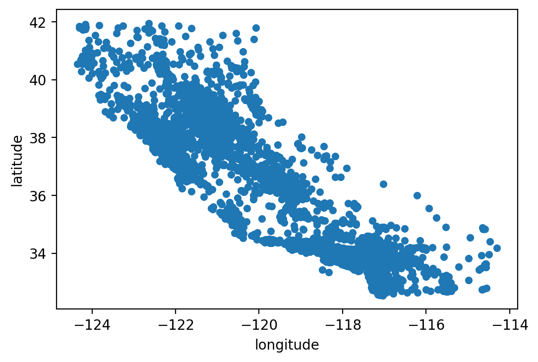
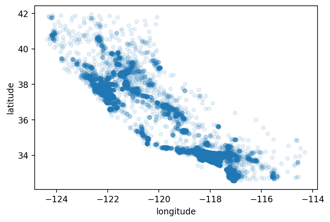
We next make a scatter splot to get a feel for the geographic location of the house observations. Once we plot it, we roughly see the outline of the State of California.
housing.plot(kind="scatter", x="longitude", y="latitude")
# save_fig("bad_visualization_plot")
<AxesSubplot:xlabel='longitude', ylabel='latitude'>
We can do a little better by making the data points in the graph a bit opaque
using the alpha option in the plot command. This option allows us to
specify the “opaqueness” of the dots in the scatterplot.
housing.plot(kind="scatter", x="longitude", y="latitude", alpha=0.1)
# save_fig("better_visualization_plot")
<AxesSubplot:xlabel='longitude', ylabel='latitude'>
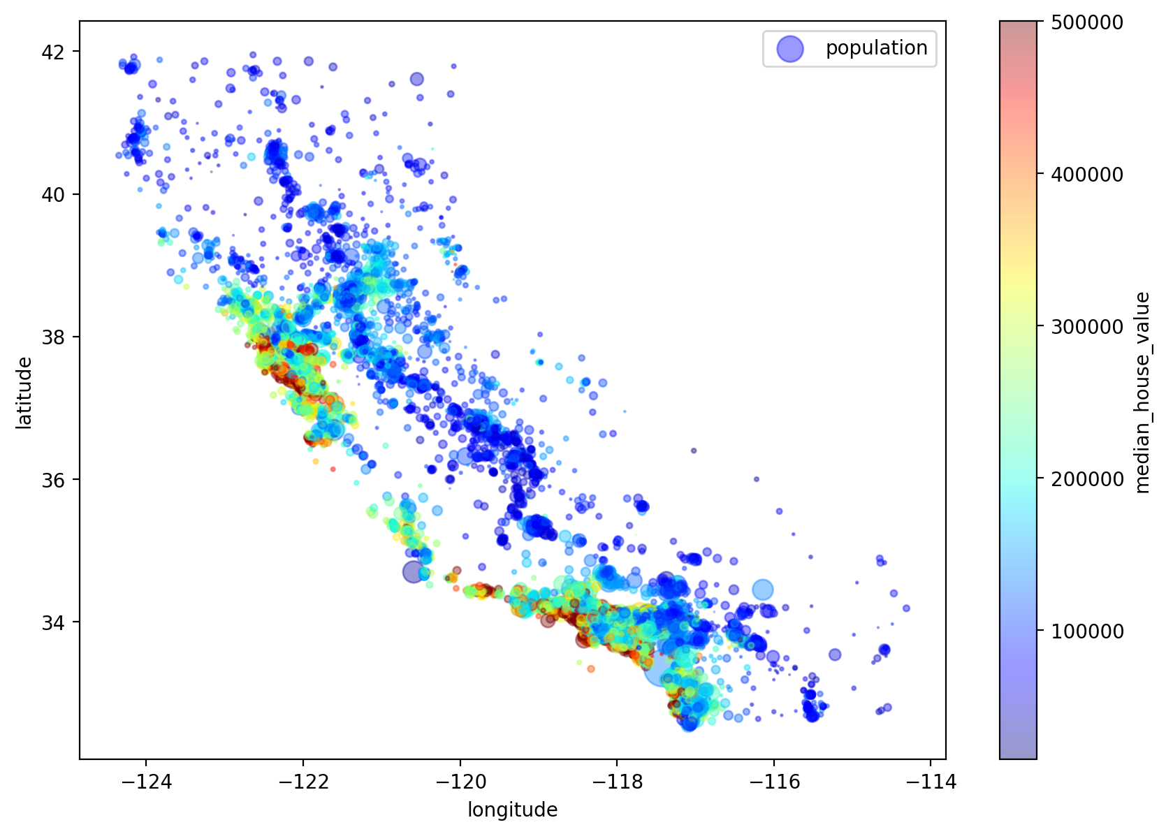
We can also adjust the data point size using a population measure. So a bigger point represents a housing observation from a place with a higher population density.
housing.plot(kind="scatter", x="longitude", y="latitude", alpha=0.4,
    s=housing["population"]/100, label="population", figsize=(10,7),
    c="median_house_value", cmap=plt.get_cmap("jet"), colorbar=True,
    sharex=False)
plt.legend()
# save_fig("housing_prices_scatterplot")
<matplotlib.legend.Legend at 0x7ff1072c59a0>
We next investigate correlations between the value of the house and the other variables in our data in order to get a feel for what a good forecasting model should factor in.
corr_matrix = housing.corr()
print(corr_matrix["median_house_value"].sort_values(ascending=False))
median_house_value    1.000000
median_income         0.687151
total_rooms           0.135140
housing_median_age    0.114146
households            0.064590
total_bedrooms        0.047781
population           -0.026882
longitude            -0.047466
latitude             -0.142673
Name: median_house_value, dtype: float64
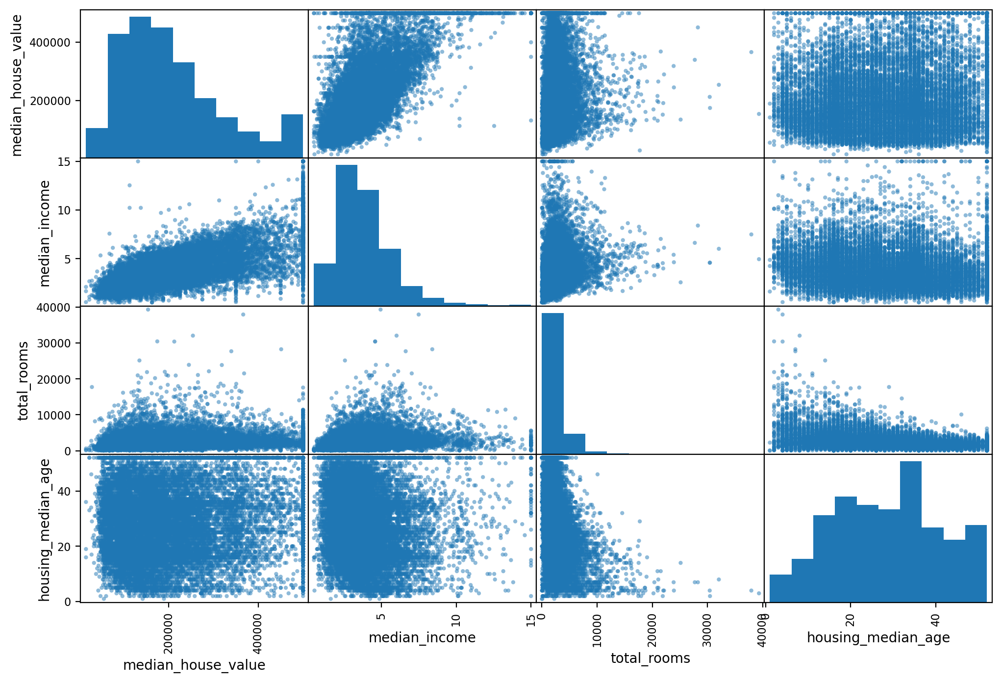
The Pandas library has a very powerful command that allows you to draw
scatter plots for all variable combinations. This is a visual method to inspect
the correlation between variables.
# from pandas.tools.plotting import scatter_matrix # For older versions of Pandas
from pandas.plotting import scatter_matrix

attributes = ["median_house_value", "median_income", "total_rooms",
              "housing_median_age"]
scatter_matrix(housing[attributes], figsize=(12, 8))
# save_fig("scatter_matrix_plot")
array([[<AxesSubplot:xlabel='median_house_value',
ylabel='median_house_value'>,
        <AxesSubplot:xlabel='median_income',
ylabel='median_house_value'>,
        <AxesSubplot:xlabel='total_rooms',
ylabel='median_house_value'>,
        <AxesSubplot:xlabel='housing_median_age',
ylabel='median_house_value'>],
       [<AxesSubplot:xlabel='median_house_value',
ylabel='median_income'>,
        <AxesSubplot:xlabel='median_income', ylabel='median_income'>,
        <AxesSubplot:xlabel='total_rooms', ylabel='median_income'>,
        <AxesSubplot:xlabel='housing_median_age',
ylabel='median_income'>],
       [<AxesSubplot:xlabel='median_house_value',
ylabel='total_rooms'>,
        <AxesSubplot:xlabel='median_income', ylabel='total_rooms'>,
        <AxesSubplot:xlabel='total_rooms', ylabel='total_rooms'>,
        <AxesSubplot:xlabel='housing_median_age',
ylabel='total_rooms'>],
       [<AxesSubplot:xlabel='median_house_value',
ylabel='housing_median_age'>,
        <AxesSubplot:xlabel='median_income',
ylabel='housing_median_age'>,
        <AxesSubplot:xlabel='total_rooms',
ylabel='housing_median_age'>,
        <AxesSubplot:xlabel='housing_median_age',
ylabel='housing_median_age'>]],
      dtype=object)
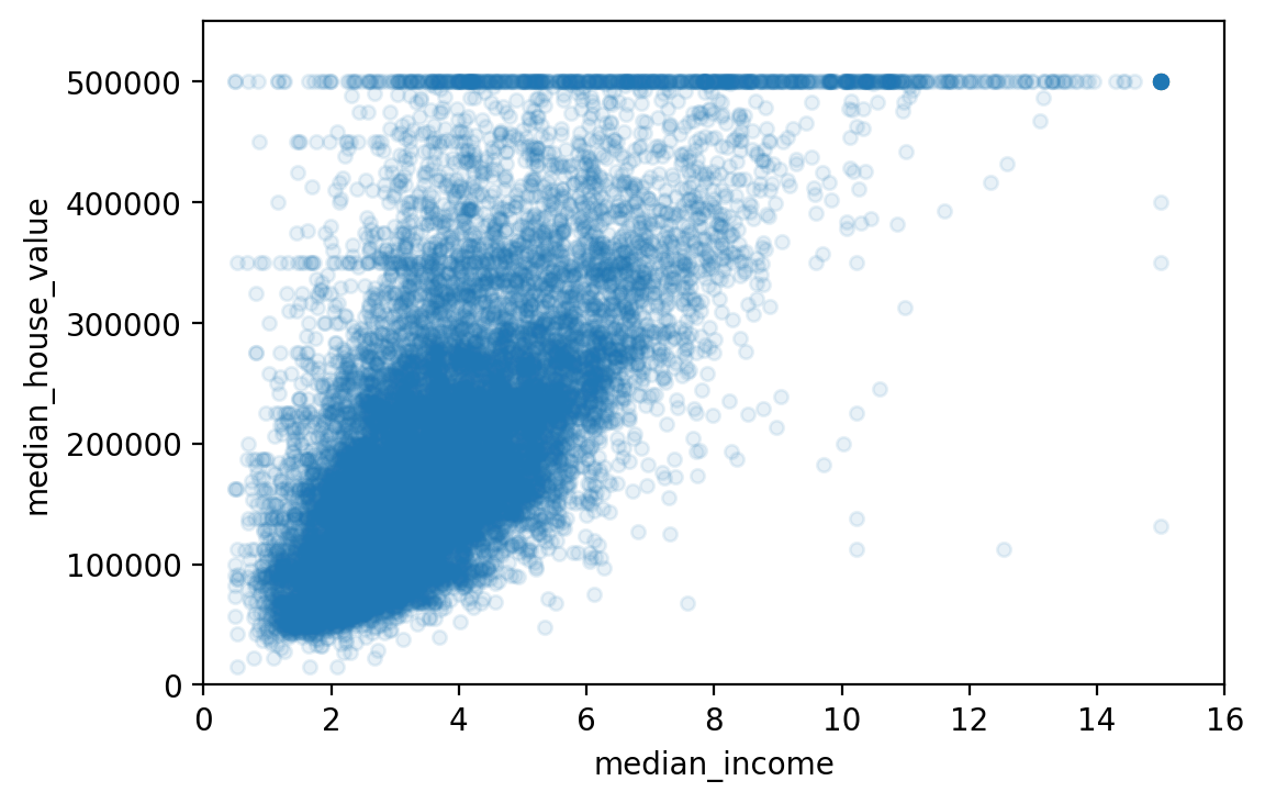
housing.plot(kind="scatter", x="median_income", y="median_house_value",
             alpha=0.1)
plt.axis([0, 16, 0, 550000])
# save_fig("income_vs_house_value_scatterplot")
(0.0, 16.0, 0.0, 550000.0)
Finally we can generate some additional variables that are combinations of variables in our original data set.
housing["rooms_per_household"] = housing["total_rooms"]/housing["households"]
housing["bedrooms_per_room"] = housing["total_bedrooms"]/housing["total_rooms"]
housing["population_per_household"]=housing["population"]/housing["households"]

# Note: there was a bug in the previous cell, in the definition of the rooms_per_household attribute. This explains why the correlation value below differs slightly from the value in the book (unless you are reading the latest version).

corr_matrix = housing.corr()
print(corr_matrix["median_house_value"].sort_values(ascending=False))
median_house_value          1.000000
median_income               0.687151
rooms_per_household         0.146255
total_rooms                 0.135140
housing_median_age          0.114146
households                  0.064590
total_bedrooms              0.047781
population_per_household   -0.021991
population                 -0.026882
longitude                  -0.047466
latitude                   -0.142673
bedrooms_per_room          -0.259952
Name: median_house_value, dtype: float64
24.2.5. Prepare data
Before training (estimating) the model we need to prepare the data for the built in Machine Learning algorithms. We need to make sure that the data only contains numeric data and not strings, lists, etc.
We first put the label variable and the rest of the data (the X variables) into separate dataframes.
housing = strat_train_set.drop("median_house_value", axis=1) # drop labels for training set
housing_labels = strat_train_set["median_house_value"].copy()
We then check how many observations with incomplete (i.e., missing) observations we have.
sample_incomplete_rows = housing[housing.isnull().any(axis=1)].head()
print(sample_incomplete_rows)
       longitude  latitude  housing_median_age  total_rooms
total_bedrooms  \
1606     -122.08     37.88                26.0       2947.0
NaN
10915    -117.87     33.73                45.0       2264.0
NaN
19150    -122.70     38.35                14.0       2313.0
NaN
4186     -118.23     34.13                48.0       1308.0
NaN
16885    -122.40     37.58                26.0       3281.0
NaN

       population  households  median_income ocean_proximity
1606        825.0       626.0         2.9330        NEAR BAY
10915      1970.0       499.0         3.4193       <1H OCEAN
19150       954.0       397.0         3.7813       <1H OCEAN
4186        835.0       294.0         4.2891       <1H OCEAN
16885      1145.0       480.0         6.3580      NEAR OCEAN
We next run a built in function over our data that attempts to impute missing data with the median values of similar observations.
# Warning: Since Scikit-Learn 0.20, the sklearn.preprocessing.Imputer class was replaced by the sklearn.impute.SimpleImputer class.
try:
    from sklearn.impute import SimpleImputer # Scikit-Learn 0.20+
except ImportError:
    from sklearn.preprocessing import Imputer as SimpleImputer

imputer = SimpleImputer(strategy="median")
Before we run the imputing algorithm we need to remove variables from the dataframe that are not numeric such as categorical variables.
Note
If you would like to use categorical variables as regressors, you need to make dummy variables for each of the categories of your categorical variable. In other words, you need to code up a categorical variable as a (dummy set of) numerical variables so that you can “do math” with your categorical variable information.
# Remove the text attribute because median can only be calculated on numerical attributes:

housing_num = housing.drop('ocean_proximity', axis=1)
# alternatively: housing_num = housing.select_dtypes(include=[np.number])
imputer.fit(housing_num)
print(imputer.statistics_)
print(housing_num.median().values)
[-118.51      34.26      29.      2119.       433.      1164.
  408.         3.54155]
[-118.51      34.26      29.      2119.       433.      1164.
  408.         3.54155]
X = imputer.transform(housing_num)

housing_tr = pd.DataFrame(X, columns=housing_num.columns,
                          index=housing.index)

print(housing_tr.head())
       longitude  latitude  housing_median_age  total_rooms
total_bedrooms  \
12655    -121.46     38.52                29.0       3873.0
797.0
15502    -117.23     33.09                 7.0       5320.0
855.0
2908     -119.04     35.37                44.0       1618.0
310.0
14053    -117.13     32.75                24.0       1877.0
519.0
20496    -118.70     34.28                27.0       3536.0
646.0

       population  households  median_income
12655      2237.0       706.0         2.1736
15502      2015.0       768.0         6.3373
2908        667.0       300.0         2.8750
14053       898.0       483.0         2.2264
20496      1837.0       580.0         4.4964
We have now created a complete dataset with no more missing observations that only contains numeric variables.
We next need to handle the categorical variable of ocean proximity of a housing unit. Let us inspect this variable first.
housing_cat = housing[['ocean_proximity']]
housing_cat.head(10)
      ocean_proximity
12655          INLAND
15502      NEAR OCEAN
2908           INLAND
14053      NEAR OCEAN
20496       <1H OCEAN
1481         NEAR BAY
18125       <1H OCEAN
5830        <1H OCEAN
17989       <1H OCEAN
4861        <1H OCEAN
We next use a label encoder function which is part of the sklearn toolkit.
This is basically a function that will generate dummy variables out of
categorical variables. Dummy variables are variables that are either 0 or 1 and
and it can be used to encode categorical (i.e., non numerical attributes) such
as gender. The dummy variable could be called d_female. It is equal to
1 if a person is female and 0 if a person is not female.
The ocean proximity variable has multiple categories in it, not just two as in
the gender example. For each category of the ocean proximity variable we have
to create a dummy variable. We could accomplish this separately for each dummy
variable using if statements or we can use the built in OrdinalEncoder
to do it in one line of code.
Warning
Some earlier machine learning codes used the LabelEncoder class or Pandas’
Series.factorize() method to encode string categorical attributes as
integers. However, the OrdinalEncoder class that was introduced in
Scikit-Learn 0.20 (see PR #10521) is preferable since it is designed for
input features (X instead of labels y) and it plays well with pipelines
(introduced later). If you are using an older version of
Scikit-Learn (<0.20), then you can import it from future_encoders.py
instead.
try:
    # New version of categorial variable encoder
    from sklearn.preprocessing import OrdinalEncoder
except ImportError:
    # Use old version, if new version of categorial variable encoder fails
    from future_encoders import OrdinalEncoder # Scikit-Learn < 0.20

ordinal_encoder = OrdinalEncoder()
housing_cat_encoded = ordinal_encoder.fit_transform(housing_cat)

print(housing_cat_encoded[:10])
print(ordinal_encoder.categories_)
[[1.]
 [4.]
 [1.]
 [4.]
 [0.]
 [3.]
 [0.]
 [0.]
 [0.]
 [0.]]
[array(['<1H OCEAN', 'INLAND', 'ISLAND', 'NEAR BAY', 'NEAR OCEAN'],
      dtype=object)]
We have now encoded a string categorical variable into numerical values.
However, before we run regressions, we need to make dummy variables out of a
categorical variable (no matter whether it’s a string category or numeric
categories). The reason is that the machine learning algorithm will assume that
two nearby values are more similar than two distant values. This is okay if
your categories are “bad”, “average”, “good”, and “excellent”, but it is not
thecase for the ocean_proximity variable above where categories 0 and 4 are
clearly more similar than categories 0 and 1.
We therefore resort to one-hot encoding, where a for each category we make a
separate variable. Let us pick one category out of the ocean_proximity
column, say “<1H OCEAN”. For this category we create a new column that we
encode as 1 (hot) if the house is less than one our from the ocean and 0(cold)
otherwise. This is also called a dummy variable.
Warning
Older machine learning codes used the LabelBinarizer or
CategoricalEncoder classes to convert each categorical value to a
one-hot vector (i.e., a dummy 0/1 variable). It is now preferable to use the
OneHotEncoder class. Since Scikit-Learn 0.20 it can
handle string categorical inputs (see PR #10521), not just integer
categorical inputs. If you are using an older version of Scikit-Learn, you
can import the new version from future_encoders.py:
try:
    from sklearn.preprocessing import OrdinalEncoder # just to raise an ImportError if Scikit-Learn < 0.20
    from sklearn.preprocessing import OneHotEncoder
except ImportError:
    from future_encoders import OneHotEncoder # Scikit-Learn < 0.20

cat_encoder = OneHotEncoder()
housing_cat_1hot = cat_encoder.fit_transform(housing_cat)

print(housing_cat_1hot)
print(cat_encoder.categories_)
  (0, 1)        1.0
  (1, 4)        1.0
  (2, 1)        1.0
  (3, 4)        1.0
  (4, 0)        1.0
  (5, 3)        1.0
  (6, 0)        1.0
  (7, 0)        1.0
  (8, 0)        1.0
  (9, 0)        1.0
  (10, 1)       1.0
  (11, 0)       1.0
  (12, 1)       1.0
  (13, 1)       1.0
  (14, 4)       1.0
  (15, 0)       1.0
  (16, 0)       1.0
  (17, 0)       1.0
  (18, 3)       1.0
  (19, 0)       1.0
  (20, 1)       1.0
  (21, 3)       1.0
  (22, 1)       1.0
  (23, 0)       1.0
  (24, 1)       1.0
  :     :
  (16487, 1)    1.0
  (16488, 0)    1.0
  (16489, 4)    1.0
  (16490, 4)    1.0
  (16491, 1)    1.0
  (16492, 1)    1.0
  (16493, 0)    1.0
  (16494, 0)    1.0
  (16495, 0)    1.0
  (16496, 1)    1.0
  (16497, 0)    1.0
  (16498, 4)    1.0
  (16499, 0)    1.0
  (16500, 0)    1.0
  (16501, 1)    1.0
  (16502, 1)    1.0
  (16503, 1)    1.0
  (16504, 1)    1.0
  (16505, 0)    1.0
  (16506, 0)    1.0
  (16507, 0)    1.0
  (16508, 1)    1.0
  (16509, 0)    1.0
  (16510, 0)    1.0
  (16511, 1)    1.0
[array(['<1H OCEAN', 'INLAND', 'ISLAND', 'NEAR BAY', 'NEAR OCEAN'],
      dtype=object)]
We next use Scikit-Learn’s FunctionTransformer class that lets you easily create a transformer based on a transformation function. Note that we need to set validate=False because the data contains non-float values (validate will default to False in Scikit-Learn 0.22).
# get the right column indices: safer than hard-coding indices 3, 4, 5, 6
rooms_ix, bedrooms_ix, population_ix, household_ix = [
    list(housing.columns).index(col)
    for col in ("total_rooms", "total_bedrooms", "population", "households")]
from sklearn.preprocessing import FunctionTransformer

def add_extra_features(X, add_bedrooms_per_room=True):
    rooms_per_household = X[:, rooms_ix] / X[:, household_ix]
    population_per_household = X[:, population_ix] / X[:, household_ix]
    if add_bedrooms_per_room:
        bedrooms_per_room = X[:, bedrooms_ix] / X[:, rooms_ix]
        return np.c_[X, rooms_per_household, population_per_household,
                     bedrooms_per_room]
    else:
        return np.c_[X, rooms_per_household, population_per_household]

attr_adder = FunctionTransformer(add_extra_features, validate=False,
                                 kw_args={"add_bedrooms_per_room": False})
housing_extra_attribs = attr_adder.fit_transform(housing.values)
print(housing_extra_attribs[0:3,:])
[[-121.46 38.52 29.0 3873.0 797.0 2237.0 706.0 2.1736 'INLAND'
  5.485835694050992 3.168555240793201]
 [-117.23 33.09 7.0 5320.0 855.0 2015.0 768.0 6.3373 'NEAR OCEAN'
  6.927083333333333 2.6236979166666665]
 [-119.04 35.37 44.0 1618.0 310.0 667.0 300.0 2.875 'INLAND'
  5.3933333333333335 2.223333333333333]]
housing_extra_attribs = pd.DataFrame(
    housing_extra_attribs,
    columns=list(housing.columns)+["rooms_per_household", "population_per_household"],
    index=housing.index)
housing_extra_attribs.head()

print(housing_extra_attribs.head())
      longitude latitude housing_median_age total_rooms total_bedrooms
\
12655   -121.46    38.52               29.0      3873.0          797.0
15502   -117.23    33.09                7.0      5320.0          855.0
2908    -119.04    35.37               44.0      1618.0          310.0
14053   -117.13    32.75               24.0      1877.0          519.0
20496    -118.7    34.28               27.0      3536.0          646.0

      population households median_income ocean_proximity
rooms_per_household  \
12655     2237.0      706.0        2.1736          INLAND
5.485836
15502     2015.0      768.0        6.3373      NEAR OCEAN
6.927083
2908       667.0      300.0         2.875          INLAND
5.393333
14053      898.0      483.0        2.2264      NEAR OCEAN
3.886128
20496     1837.0      580.0        4.4964       <1H OCEAN
6.096552

      population_per_household
12655                 3.168555
15502                 2.623698
2908                  2.223333
14053                 1.859213
20496                 3.167241
from sklearn.pipeline import Pipeline
from sklearn.preprocessing import StandardScaler

num_pipeline = Pipeline([
        ('imputer', SimpleImputer(strategy="median")),
        ('attribs_adder', FunctionTransformer(add_extra_features, validate=False)),
        ('std_scaler', StandardScaler()),
    ])

housing_num_tr = num_pipeline.fit_transform(housing_num)
try:
    from sklearn.compose import ColumnTransformer
except ImportError:
    from future_encoders import ColumnTransformer # Scikit-Learn < 0.20


num_attribs = list(housing_num)
cat_attribs = ["ocean_proximity"]

full_pipeline = ColumnTransformer([
        ("num", num_pipeline, num_attribs),
        ("cat", OneHotEncoder(), cat_attribs),
    ])

housing_prepared = full_pipeline.fit_transform(housing)
print(housing_prepared[:3,:])
[[-0.94135046  1.34743822  0.02756357  0.58477745  0.64037127
0.73260236
   0.55628602 -0.8936472   0.01739526  0.00622264 -0.12112176  0.
   1.          0.          0.          0.        ]
 [ 1.17178212 -1.19243966 -1.72201763  1.26146668  0.78156132
0.53361152
   0.72131799  1.292168    0.56925554 -0.04081077 -0.81086696  0.
   0.          0.          0.          1.        ]
 [ 0.26758118 -0.1259716   1.22045984 -0.46977281 -0.54513828
-0.67467519
  -0.52440722 -0.52543365 -0.01802432 -0.07537122 -0.33827252  0.
   1.          0.          0.          0.        ]]
24.2.6. Training a Regression Model
#%% Select and train a model

from sklearn.linear_model import LinearRegression

lin_reg = LinearRegression()
lin_reg.fit(housing_prepared, housing_labels)

# let's try the full preprocessing pipeline on a few training instances
some_data = housing.iloc[:5]
some_labels = housing_labels.iloc[:5]
some_data_prepared = full_pipeline.transform(some_data)

print("Predictions:", lin_reg.predict(some_data_prepared))
print("Lables:", list(some_labels))
Predictions: [ 85657.90192014 305492.60737488 152056.46122456
186095.70946094
 244550.67966089]
Lables: [72100.0, 279600.0, 82700.0, 112500.0, 238300.0]
from sklearn.metrics import mean_squared_error

housing_predictions = lin_reg.predict(housing_prepared)
lin_mse = mean_squared_error(housing_labels, housing_predictions)
lin_rmse = np.sqrt(lin_mse)
print(lin_rmse)
68627.87390018743
from sklearn.metrics import mean_absolute_error

lin_mae = mean_absolute_error(housing_labels, housing_predictions)
print(lin_mae)
49438.66860915803
from sklearn.tree import DecisionTreeRegressor

tree_reg = DecisionTreeRegressor(random_state=42)
tree_reg.fit(housing_prepared, housing_labels)

DecisionTreeRegressor(criterion='mse', max_depth=None, max_features=None,
           max_leaf_nodes=None, min_impurity_decrease=0.0,
           min_impurity_split=None, min_samples_leaf=1,
           min_samples_split=2, min_weight_fraction_leaf=0.0,
           presort=False, random_state=42, splitter='best')

housing_predictions = tree_reg.predict(housing_prepared)
tree_mse = mean_squared_error(housing_labels, housing_predictions)
tree_rmse = np.sqrt(tree_mse)
print(tree_rmse)
---------------------------------------------------------------------------TypeError
Traceback (most recent call last)/tmp/ipykernel_8088/2927567427.py in
<module>
      4 tree_reg.fit(housing_prepared, housing_labels)
      5
----> 6 DecisionTreeRegressor(criterion='mse', max_depth=None,
max_features=None,
      7            max_leaf_nodes=None, min_impurity_decrease=0.0,
      8            min_impurity_split=None, min_samples_leaf=1,
TypeError: __init__() got an unexpected keyword argument
'min_impurity_split'
from sklearn.model_selection import cross_val_score

scores = cross_val_score(tree_reg, housing_prepared, housing_labels,
                         scoring="neg_mean_squared_error", cv=10)
tree_rmse_scores = np.sqrt(-scores)

def f_display_scores(scores):
    print("Scores:", scores)
    print("Mean:", scores.mean())
    print("Standard deviation:", scores.std())

f_display_scores(tree_rmse_scores)
Scores: [72831.45749112 69973.18438322 69528.56551415 72517.78229792
 69145.50006909 79094.74123727 68960.045444   73344.50225684
 69826.02473916 71077.09753998]
Mean: 71629.89009727491
Standard deviation: 2914.035468468928
lin_scores = cross_val_score(lin_reg, housing_prepared, housing_labels,
                             scoring="neg_mean_squared_error", cv=10)
lin_rmse_scores = np.sqrt(-lin_scores)
f_display_scores(lin_rmse_scores)
Scores: [71762.76364394 64114.99166359 67771.17124356 68635.19072082
 66846.14089488 72528.03725385 73997.08050233 68802.33629334
 66443.28836884 70139.79923956]
Mean: 69104.07998247063
Standard deviation: 2880.328209818062
# Note: we specify n_estimators=10 to avoid a warning about the fact that the default value is going to change to 100 in Scikit-Learn 0.22.
from sklearn.ensemble import RandomForestRegressor

forest_reg = RandomForestRegressor(n_estimators=10, random_state=42)
forest_reg.fit(housing_prepared, housing_labels)


housing_predictions = forest_reg.predict(housing_prepared)
forest_mse = mean_squared_error(housing_labels, housing_predictions)
forest_rmse = np.sqrt(forest_mse)
print(forest_rmse)
22413.454658589766
from sklearn.model_selection import cross_val_score

forest_scores = cross_val_score(forest_reg, housing_prepared, housing_labels,
                                scoring="neg_mean_squared_error", cv=10)
forest_rmse_scores = np.sqrt(-forest_scores)
f_display_scores(forest_rmse_scores)


scores = cross_val_score(lin_reg, housing_prepared, housing_labels, scoring="neg_mean_squared_error", cv=10)
pd.Series(np.sqrt(-scores)).describe()
Scores: [53519.05518628 50467.33817051 48924.16513902 53771.72056856
 50810.90996358 54876.09682033 56012.79985518 52256.88927227
 51527.73185039 55762.56008531]
Mean: 52792.92669114079
Standard deviation: 2262.8151900582
count       10.000000
mean     69104.079982
std       3036.132517
min      64114.991664
25%      67077.398482
50%      68718.763507
75%      71357.022543
max      73997.080502
dtype: float64
24.2.7. Fine Tune Model
from sklearn.model_selection import GridSearchCV

param_grid = [
    # try 12 (3×4) combinations of hyperparameters
    {'n_estimators': [3, 10, 30], 'max_features': [2, 4, 6, 8]},
    # then try 6 (2×3) combinations with bootstrap set as False
    {'bootstrap': [False], 'n_estimators': [3, 10], 'max_features': [2, 3, 4]},
  ]

forest_reg = RandomForestRegressor(random_state=42)
# train across 5 folds, that's a total of (12+6)*5=90 rounds of training
grid_search = GridSearchCV(forest_reg, param_grid, cv=5,
                           scoring='neg_mean_squared_error', return_train_score=True)
grid_search.fit(housing_prepared, housing_labels)

print(grid_search.best_params_)
{'max_features': 8, 'n_estimators': 30}
print(grid_search.best_estimator_)
RandomForestRegressor(max_features=8, n_estimators=30,
random_state=42)
# Let's look at the score of each hyperparameter combination tested during the grid search:
cvres = grid_search.cv_results_

for mean_score, params in zip(cvres["mean_test_score"], cvres["params"]):
    print(np.sqrt(-mean_score), params)
63895.161577951665 {'max_features': 2, 'n_estimators': 3}
54916.32386349543 {'max_features': 2, 'n_estimators': 10}
52885.86715332332 {'max_features': 2, 'n_estimators': 30}
60075.3680329983 {'max_features': 4, 'n_estimators': 3}
52495.01284985185 {'max_features': 4, 'n_estimators': 10}
50187.24324926565 {'max_features': 4, 'n_estimators': 30}
58064.73529982314 {'max_features': 6, 'n_estimators': 3}
51519.32062366315 {'max_features': 6, 'n_estimators': 10}
49969.80441627874 {'max_features': 6, 'n_estimators': 30}
58895.824998155826 {'max_features': 8, 'n_estimators': 3}
52459.79624724529 {'max_features': 8, 'n_estimators': 10}
49898.98913455217 {'max_features': 8, 'n_estimators': 30}
62381.765106921855 {'bootstrap': False, 'max_features': 2,
'n_estimators': 3}
54476.57050944266 {'bootstrap': False, 'max_features': 2,
'n_estimators': 10}
59974.60028085155 {'bootstrap': False, 'max_features': 3,
'n_estimators': 3}
52754.5632813202 {'bootstrap': False, 'max_features': 3,
'n_estimators': 10}
57831.136061214274 {'bootstrap': False, 'max_features': 4,
'n_estimators': 3}
51278.37877140253 {'bootstrap': False, 'max_features': 4,
'n_estimators': 10}
feature_importances = grid_search.best_estimator_.feature_importances_
print(feature_importances)
[6.96542523e-02 6.04213840e-02 4.21882202e-02 1.52450557e-02
 1.55545295e-02 1.58491147e-02 1.49346552e-02 3.79009225e-01
 5.47789150e-02 1.07031322e-01 4.82031213e-02 6.79266007e-03
 1.65706303e-01 7.83480660e-05 1.52473276e-03 3.02816106e-03]
extra_attribs = ["rooms_per_hhold", "pop_per_hhold", "bedrooms_per_room"]
#cat_encoder = cat_pipeline.named_steps["cat_encoder"] # old solution
cat_encoder = full_pipeline.named_transformers_["cat"]
cat_one_hot_attribs = list(cat_encoder.categories_[0])
attributes = num_attribs + extra_attribs + cat_one_hot_attribs
sorted(zip(feature_importances, attributes), reverse=True)

final_model = grid_search.best_estimator_

X_test = strat_test_set.drop("median_house_value", axis=1)
y_test = strat_test_set["median_house_value"].copy()

X_test_prepared = full_pipeline.transform(X_test)
final_predictions = final_model.predict(X_test_prepared)

final_mse = mean_squared_error(y_test, final_predictions)
final_rmse = np.sqrt(final_mse)
print(final_rmse)
47873.26095812988
from scipy import stats

confidence = 0.95
squared_errors = (final_predictions - y_test) ** 2
mean = squared_errors.mean()
m = len(squared_errors)

CI = np.sqrt(stats.t.interval(confidence, m - 1,
                         loc=np.mean(squared_errors),
                         scale=stats.sem(squared_errors)))

print("Confidence Interval", CI)
Confidence Interval [45893.36082829 49774.46796717]
24.3. Key Concepts and Summary
Note
Machine learning
The basics