19. Optimization
In this section I introduce algorithms that can find the minimum or maximum of a function. I will rely heavily on the previous chapter on root-finding. Many optimization problem can be recast as root-finding problems of the first derivative of the function that needs to be optimized.
As you have already noticed this book teaches by example. I will therefore first introduce the function that we will try “to optimize.”
19.1. Univariate Function Optimization
import numpy as np
import matplotlib.pyplot as plt
import math as m
import time  # Imports system time module to time your script

plt.close('all')  # close all open figures
Here we want to optimize a univariate function:
Think of it as a profit function of a company, where the argument of the function, the \(x\), is the amount of goods produced and subsequently sold. The more you produce and sell i.e., the larger the \(x\) gets, the more profit you will make. But only up to a point. If you overdo it and start to produce too much, inefficiencies in production start to creep in possibly due to congestion in the production process or not enough demand so that production becomes wasteful and costlier the more you keep on producing. In other words, there is a sweet spot that you should not cross and if you do your profits will actually go down.
In Python we first define the function:
def f_profit(x):
    if (x < 0):
        return (0)
    if (x == 0):
        return (np.nan)
    y = np.exp(-2*x)
    return (4 * x**2 * y)
Notice that I put a check into the function that returns zero for negative \(x\) values. You cannot produce negative amounts, so we need to take care of this here.
Second I put a check in for zero value. Since you have a negative exponent, and x of zero would lead to a division by zero which usually breaks the code and returns a “division-by-zero” error. Mathematically a division by zero result in infinity. Infinity is not a problem for mathematical theory but it is a problem for numerical computation. We want to avoid it.
Plotting the function is always a good idea!
xmin = 0.0
xmax = 6.0
xv = np.arange(xmin, xmax, (xmax - xmin)/200.0)
fx = np.zeros(len(xv),float) # define column vector
for i in range(len(xv)):
    fx[i] = f_profit(xv[i])

fig, ax = plt.subplots()
ax.plot(xv, fx)
ax.plot(xv, np.zeros(len(xv)))
ax.set_xlabel('x')
ax.set_ylabel('f(x)')
ax.set_title('Profit Function')
plt.show()
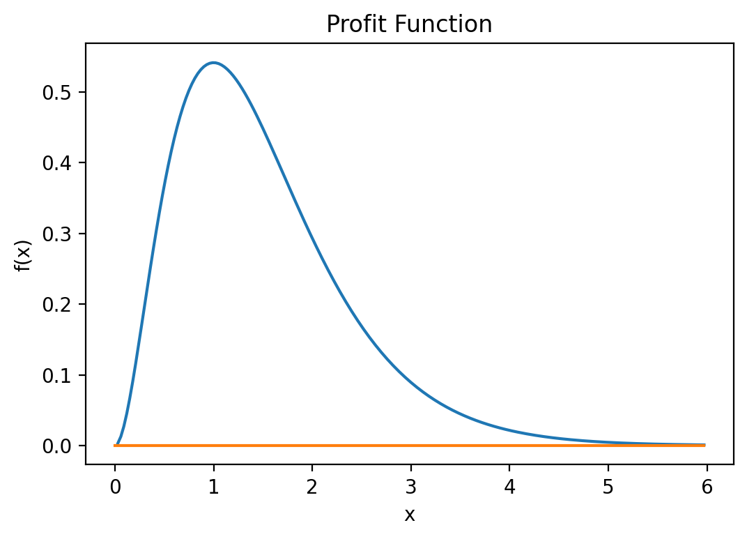
From the plot we see that this function seems to have a maximum around when \(x \approx 1.0\). It also seems to be the only maximum which would make it a global maximum.
19.2. Optimization Methods
19.2.1. Newton’s Method
What do we know is true at the maximum? If you draw tangent lines along the function, we know that the tangent line at the maximum (or peak) of the function is a flat line. Like so:
xmin = 0.0
xmax = 6.0
xv = np.linspace(xmin, xmax, 200)
fx = np.zeros(len(xv),float) # define column vector
for i in range(len(xv)):
    fx[i] = f_profit(xv[i])

fig, ax = plt.subplots()
ax.plot(xv, fx)
ax.plot(xv, f_profit(1)*np.ones(len(xv)))
ax.set_xlabel('x')
ax.set_ylabel('f(x)')
ax.set_title('Profit Function')
plt.show()
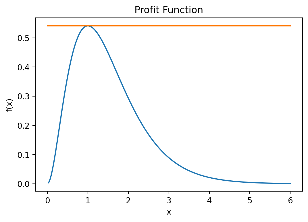
Is there a mathematical expression for a tangent line? Yes there is, it is called the first derivative. This means that at the peak (i.e., maximum) of the function, the slope of the derivative is zero, right?
In other words, if we can find the \(x\) value where the derivate of the function evaluates to zero, or \(f'(x) = 0\), then we would have found the \(x\) value where the function is at its maximum value.
Let’s plot the derivative then and see where its value is zero. Calculus first. Derive the function and you will have:
Derive it again (you will see shortly why) and you will get the second derivative:
Next we define another Python function that returns all three, the function value \(f(x)\), the value of the derivative \(f'(x)\), and the value of the second derivative \(f''(x)\). Those are required by some of the algorithms that you are going to see shortly.
def f_profit_plus_deriv(x):
    # gamma(2,3) density
    if (x < 0):
        return np.array([0, 0, 0])
    if (x == 0):
        return np.array([0, 0, np.nan])
    y = np.exp(-2.0*x)
    return np.array([4.0 * x**2.0 * np.exp(-2.0*x), \
      8.0 * np.exp(-2.0*x) * x*(1.0-x), \
      8.0 * np.exp(-2.0*x) * (1 - 4*x + 2 * x**2)])
xmin = 0.0
xmax = 6.0
xv = np.linspace(xmin, xmax, 200)
dfx = np.zeros(len(xv),float) # define column vector
for i in range(len(xv)):

    # The derivate value is in the second position
    dfx[i] = f_profit_plus_deriv(xv[i])[1]

fig, ax = plt.subplots()
ax.plot(xv, dfx)
ax.plot(xv, 0*np.ones(len(xv)))
ax.set_xlabel('x')
ax.set_ylabel('f\'(x)')
ax.set_title('Derivative of Profit Function')
plt.show()
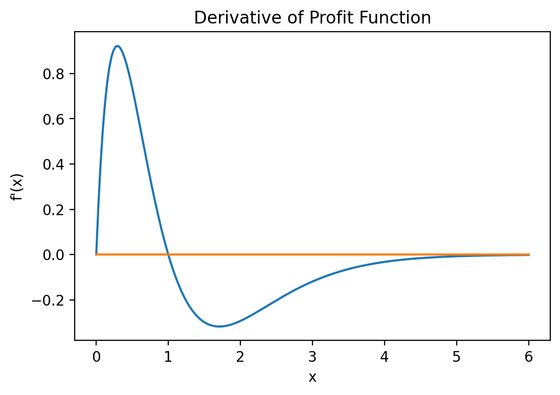
From this plot we see that the derivate function crosses the horizontal axis at and \(x\) value of, well, one. So I gave it away, the maximum of the function is at \(x=1\).
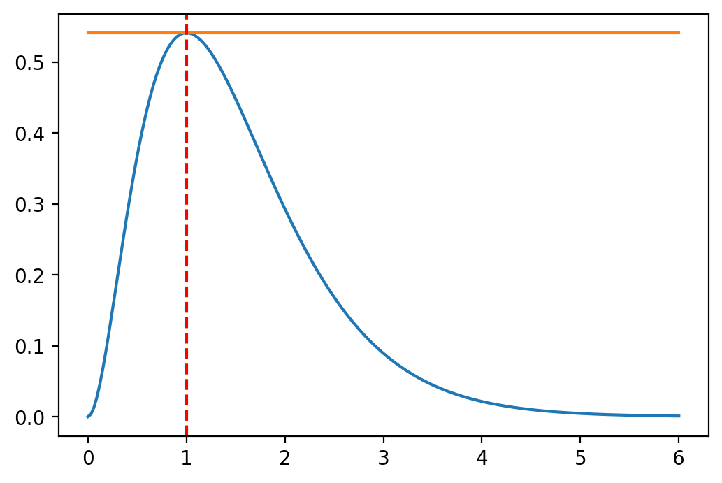
Let us pretend for a minute that we do not know that or are not entirely sure whether this is really our maximum value and let us therefore use the Newton algorithm from the previous chapter to make sure that the root of the derivative function is really at one. In order to implement the Newton method we basically look for the root of a first derivative so that \(f'(x) = 0\).
myOpt = 1.0
fmaxval = f_profit(myOpt)

xmin = 0.0
xmax = 6.0
xv = np.linspace(xmin, xmax, 200)
fx = np.zeros(len(xv),float) # define column vector
for i in range(len(xv)):
    fx[i] = f_profit_plus_deriv(xv[i])[0]

fig, ax = plt.subplots()
ax.plot(xv, fx)
ax.plot(xv, fmaxval*np.ones(len(xv)))
ax.axvline(x = myOpt, ymin=0.0, color='r', linestyle='--')
plt.show()
We then use the root finding algorithm from the previous chapter to find this point, or:
Note
Newthon-Raphson Root Finding Algorithm
We have to adjust this of course because the function we search the foot for is already the first derivative of a function, so that we have:
\[x_{n+1} = x_n - \frac{f'(x_n)}{f''(x_n)}\]
def newton(f3, x0, tol = 1e-9, nmax = 100):
    # Newton's method for optimization, starting at x0
    # f3 is a function that given x returns the vector
    # (f(x), f'(x), f''(x)), for some f
    x = x0
    f3v = f3(x)
    n = 0
    while ((abs(f3v[1]) > tol) and (n < nmax)):
        # 1st derivative value is the second return value
        # 2nd derivative value is the third return value
        x = x - f3v[1]/f3v[2]
        f3v = f3(x)
        n = n + 1
    if (n == nmax):
        print("newton failed to converge")
    else:
        return(x)
We next use these algorithms to find the maximum point of our function f_profit_plus_deriv
and f_profit. Note that if we use the Newton algorithm we will need the
first and second derivatives of the functions. This is why we use function
f_profit_plus_deriv that returns f, f' and f'' via an array/vector as return value.
print(" -----------------------------------")
print(" Newton results ")
print(" -----------------------------------")
print(newton(f_profit_plus_deriv, 0.25))
print(newton(f_profit_plus_deriv, 0.5))
print(newton(f_profit_plus_deriv, 0.75))
print(newton(f_profit_plus_deriv, 1.75))
 -----------------------------------
 Newton results
 -----------------------------------
-1.25
1.0
0.9999999999980214
14.42367881581733
19.2.2. Golden Section Method
The golden-section method works in one dimension only, but does not need the derivatives of the function. However, the function still needs to be continuous. In order to determine whether there is a local maximum we need three points. Then we can use the following:
Note
If \(x_l<x_m<x_r\) and
\(f(x_l) \leq f(x_m)\) and
\(f(x_r) \leq f(x_m)\) then there
must be a local maximum in the interval between \([x_l,x_r].\)
This method is very similar to the bisection method (root bracketing) from the previous section.
The method starts with three starting values and operates by successively narrowing the range of values on the specified interval, which makes it relatively slow, but very robust. The technique derives its name from the fact that the algorithm maintains the function values for four points whose three interval widths are in the ratio
where \(\rho\) is the golden ratio.
In mathematics, two quantities \(a\) and \(b\) are in the golden ratio if their ratio is the same as the ratio of their sum to the larger of the two quantities. Assume \(a>b\) then the ratio:
Fig. 19.1 illustrates this geometric relationship.
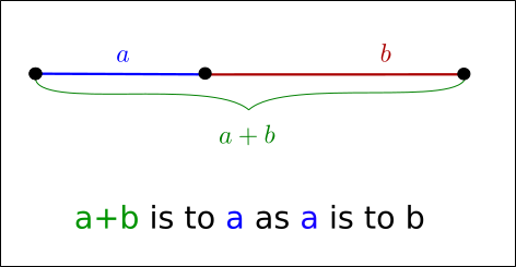
Fig. 19.1 Line segments in the golden ratio
The golden ratio is the solution to:
so that
The algorithm proceeds in the following way:
Note
Start with \(x_l<x_m<x_r\) such that
and
and the golden ratio
In the algorithm we then check the following:
If \(x_r - x_l \le \epsilon\) then stop
If \(x_r-x_m > x_m-x_l\) then do \((a)\) otherwise do \((b)\)
Let \(y=x_m+(x_r-x_m)/(1+\rho)\) if \(f(y) \ge f(x_m)\) then put \(x_l=x_m\) and \(x_m=y\) otherwise put \(x_r=y\)
Let \(y=x_m+(x_m-x_l)/(1+\rho)\) if \(f(y) \ge f(x_m)\) then put \(x_r=x_m\) and \(x_m=y\) otherwise put \(x_l=y\)
Go back to step 1
Fig. 19.2 illustrates a maximization problem set up according to the golden ratio algorithm.
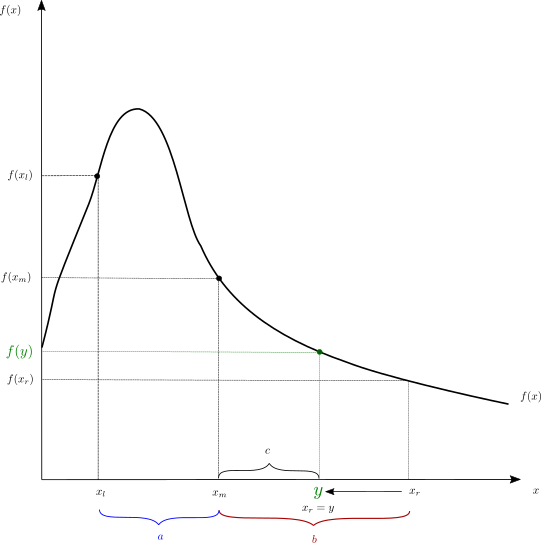
Fig. 19.2 Maximization using the Golden Ratio Algorithm
def gsection(ftn, xl, xm, xr, tol = 1e-9):
    # applies the golden-section algorithm to maximise ftn
    # we assume that ftn is a function of a single variable
    # and that x.l < x.m < x.r and ftn(x.l), ftn(x.r) <= ftn(x.m)
    #
    # the algorithm iteratively refines x.l, x.r, and x.m and
    # terminates when x.r - x.l <= tol, then returns x.m
    # golden ratio plus one
    gr1 = 1 + (1 + np.sqrt(5))/2
    #
    # successively refine x.l, x.r, and x.m
    fl = ftn(xl)
    fr = ftn(xr)
    fm = ftn(xm)
    while ((xr - xl) > tol):
        if ((xr - xm) > (xm - xl)):
            y = xm + (xr - xm)/gr1
            fy = ftn(y)
            if (fy >= fm):
                xl = xm
                fl = fm
                xm = y
                fm = fy
            else:
                xr = y
                fr = fy
        else:
            y = xm - (xm - xl)/gr1
            fy = ftn(y)
            if (fy >= fm):
                xr = xm
                fr = fm
                xm = y
                fm = fy
            else:
                xl = y
                fl = fy
    return(xm)
The Golden section algorithm does not require the derivates of the function, so
we just call the f_profit function that only returns the functional value.
print(" -----------------------------------")
print(" Golden section results ")
print(" -----------------------------------")
myOpt = gsection(f_profit, 0.1, 0.25, 1.3)
print(gsection(f_profit, 0.1, 0.25, 1.3))
print(gsection(f_profit, 0.25, 0.5, 1.7))
print(gsection(f_profit, 0.6, 0.75, 1.8))
print(gsection(f_profit, 0.0, 2.75, 5.0))
 -----------------------------------
 Golden section results
 -----------------------------------
1.0000000117853984
1.0000000107340477
0.9999999921384167
1.0000000052246139
19.2.3. Use Built-In Method to Maximize Function
Finally, we can also use a built in function minimizer.
The built in function fmin is in the scipy.optimize library. We need to
import it first. So if we want to maximize our function we have to define it
as a negated function, that is:
then
is the same as
Since we want to find the maximum of the function, we need to “trick” the minimization algorithm. We therefore need to redefine the function as
def f_profitNeg(x):
    # gamma(2,3) density
    if (x < 0):
        return (0)
    if (x == 0):
        return (np.nan)
    y = np.exp(-2*x)
    return (-(4 * x**2 * y))
Here we simply return negative values of this function. If we now minimize this function, we actually maximize the original function
from scipy.optimize import fmin

print(" -----------------------------------")
print(" fmin results ")
print(" -----------------------------------")
print(fmin(f_profitNeg, 0.25))
print(fmin(f_profitNeg, 0.5))
print(fmin(f_profitNeg, 0.75))
print(fmin(f_profitNeg, 1.75))
 -----------------------------------
 fmin results
 -----------------------------------
Optimization terminated successfully.
         Current function value: -0.541341
         Iterations: 18
         Function evaluations: 36
[1.]
Optimization terminated successfully.
         Current function value: -0.541341
         Iterations: 16
         Function evaluations: 32
[1.]
Optimization terminated successfully.
         Current function value: -0.541341
         Iterations: 14
         Function evaluations: 28
[0.99997559]
Optimization terminated successfully.
         Current function value: -0.541341
         Iterations: 16
         Function evaluations: 32
[1.00001221]
19.3. Finding the Root of a Function using Minimization
In a previous chapter on root searching of a function we used various methods like the built in fsolve or root functions from the scipy.optimize library. Here’s the example from the Root finding chapter again:
The example function for which we calculate the root, i.e., find \(x\) so that \(f(x) = 0\) is defined as:
def func(x):
    s = np.log(x) - np.exp(-x)  # function: f(x)
    return s
We can solve for the zero (root) position with:
from scipy.optimize import root

guess = 2
result = root(func, guess) # starting from x = 2
print(" ")
print(" -------------- Root ------------")
myroot = result.x  # Grab number from result dictionary
print("The root of d_func is at {}".format(myroot))
print("The max value of the function is {}".format(myOpt))
 -------------- Root ------------
The root of d_func is at [1.30979959]
The max value of the function is 1.0000000117853984
In this section we set up the root finding problem as an optimization problem. In order to do this we change the return value of the function slightly to
So we are trying to find the value of
x so that the residual error between \(f(x)\) and its target value of
\(0\) is as small as possible. The new function is defined as:
def func_root_min(x):
    s = np.log(x) - np.exp(-x)  # function: f(x)
    return (s**2)
We now invoke a minimizing algorithm to find this value of \(x\)
from scipy.optimize import minimize

guess = 2 # starting guess x = 2
result = minimize(func_root_min, guess, method='Nelder-Mead')

print(" ")
print("-------------- Root ------------")
myroot = result.x  # Grab number from result dictionary
print("The root of func is at {}".format(myroot))
-------------- Root ------------
The root of func is at [1.30976562]
19.4. Multivariate Optimization
19.4.1. Function
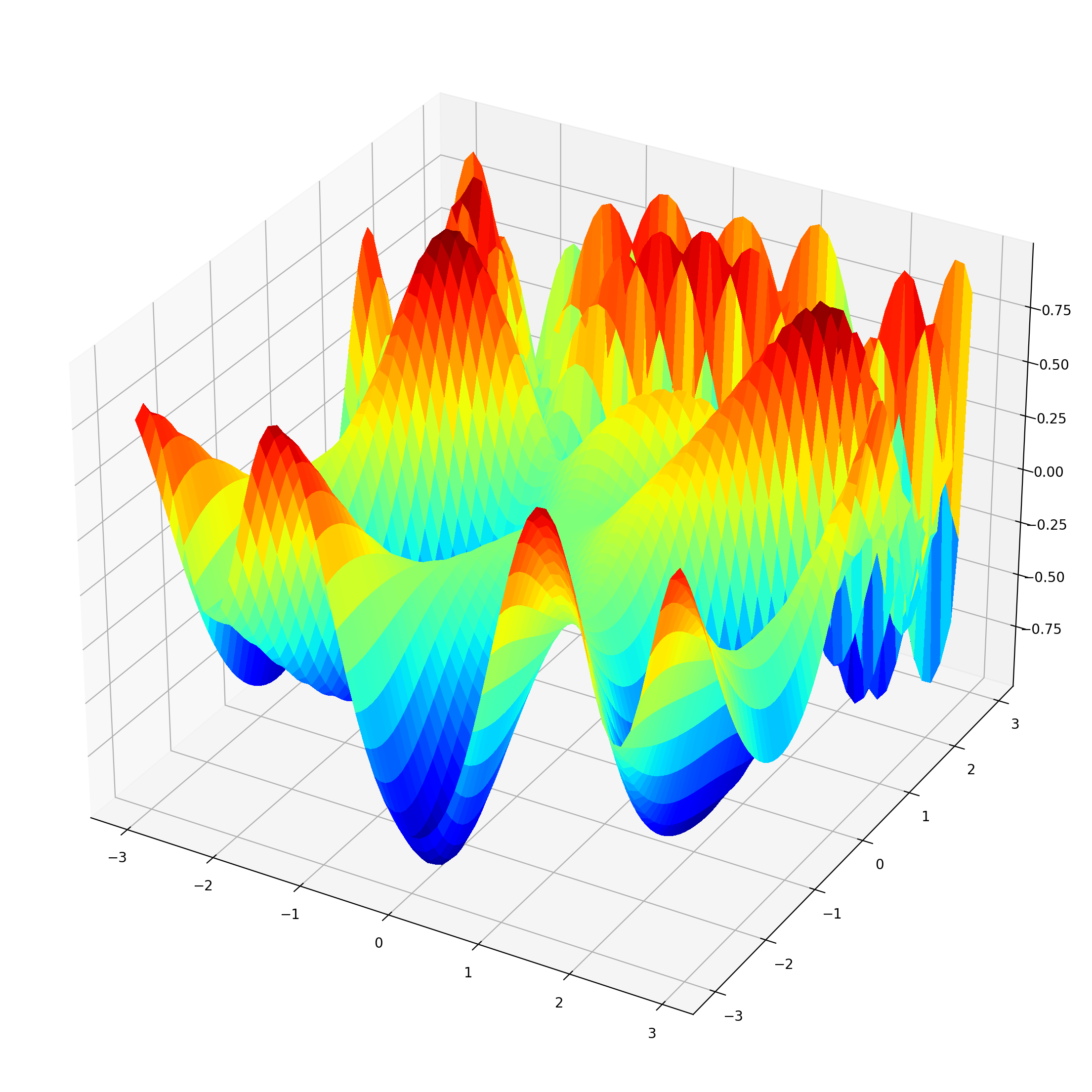
Here we want to optimize the following function f3
def f3simple(x):
    a = x[0]**2/2.0 - x[1]**2/4.0
    b = 2*x[0] - np.exp(x[1])
    f = np.sin(a)*np.cos(b)
    return(f)
Its negative version:
def f3simpleNeg(x):
    a = x[0]**2/2.0 - x[1]**2/4.0
    b = 2*x[0] - np.exp(x[1])
    f = -np.sin(a)*np.cos(b)
    return(f)
And the version that returns \(f(x)\), \(f'(x)\) (i.e., the gradient), and \(f''(x)\) (i.e., the Hessian matrix):
def f3(x):
    a = x[0]**2/2.0 - x[1]**2/4.0
    b = 2*x[0] - np.exp(x[1])
    f = np.sin(a)*np.cos(b)
    f1 = np.cos(a)*np.cos(b)*x[0] - np.sin(a)*np.sin(b)*2
    f2 = -np.cos(a)*np.cos(b)*x[1]/2 + np.sin(a)*np.sin(b)*np.exp(x[1])
    f11 = -np.sin(a)*np.cos(b)*(4 + x[0]**2) + np.cos(a)*np.cos(b) \
        - np.cos(a)*np.sin(b)*4*x[0]
    f12 = np.sin(a)*np.cos(b)*(x[0]*x[1]/2.0 + 2*np.exp(x[1])) \
        + np.cos(a)*np.sin(b)*(x[0]*np.exp(x[1]) + x[1])
    f22 = -np.sin(a)*np.cos(b)*(x[1]**2/4.0 + np.exp(2*x[1])) \
        - np.cos(a)*np.cos(b)/2.0 - np.cos(a)*np.sin(b)*x[1]*np.exp(x[1]) \
        + np.sin(a)*np.sin(b)*np.exp(x[1])
    # Function f3 returns: f(x), f'(x), and f''(x)
    return (f, np.array([f1, f2]), np.array([[f11, f12], [f12, f22]]))
We next plot the function:
from mpl_toolkits.mplot3d import Axes3D

fig = plt.figure(figsize=(14, 16))
ax = plt.gca(projection='3d')

X = np.arange(-3, 3, .1)
Y = np.arange(-3, 3, .1)
X, Y = np.meshgrid(X, Y)

Z = np.zeros((len(X),len(Y)),float)
for i in range(len(X)):
    for j in range(len(Y)):
        Z[i][j] = f3simple([X[i][j],Y[i][j]])

surf = ax.plot_surface(X, Y, Z, rstride=1, cstride=1, \
    cmap=plt.cm.jet, linewidth=0, antialiased=False)
plt.show()
/tmp/ipykernel_40767/2176093652.py:4: MatplotlibDeprecationWarning:
Calling gca() with keyword arguments was deprecated in Matplotlib 3.4.
Starting two minor releases later, gca() will take no keyword
arguments. The gca() function should only be used to get the current
axes, or if no axes exist, create new axes with default keyword
arguments. To create a new axes with non-default arguments, use
plt.axes() or plt.subplot().
  ax = plt.gca(projection='3d')
19.4.2. Multivariate Newton Method
def newtonMult(f3, x0, tol = 1e-9, nmax = 100):
    # Newton's method for optimization, starting at x0
    # f3 is a function that given x returns the list
    # {f(x), grad f(x), Hessian f(x)}, for some f
    x = x0
    f3x = f3(x)
    n = 0
    while ((max(abs(f3x[1])) > tol) and (n < nmax)):
        x = x - np.linalg.solve(f3x[2], f3x[1])
        f3x = f3(x)
        n = n + 1
    if (n == nmax):
        print("newton failed to converge")
    else:
        return(x)
Compare the Newton method with the built in fmin method in
scipy.optimize. We use various starting values to see whether we can find
more than one optimum.
from scipy.optimize import fmin

for x0 in np.arange(1.4, 1.6, 0.1):
    for y0 in np.arange(0.4, 0.7, 0.1):
        # This algorithm requires f(x), f'(x), and f''(x)
        print("Newton: f3  " + str([x0,y0]) + ' --> ' + str(newtonMult(f3, \
            np. array([x0,y0]))))

        print("fmin: f3 " + str([x0,y0]) + ' --> ' \
            + str(fmin(f3simpleNeg, np.array([x0,y0]))))

        print(" ----------------------------------------- ")
Newton: f3  [1.4, 0.4] --> [ 0.04074437 -2.50729047]
Optimization terminated successfully.
         Current function value: -1.000000
         Iterations: 47
         Function evaluations: 89
fmin: f3 [1.4, 0.4] --> [2.0307334  1.40155445]
 -----------------------------------------
Newton: f3  [1.4, 0.5] --> [0.11797341 3.34466147]
Optimization terminated successfully.
         Current function value: -1.000000
         Iterations: 50
         Function evaluations: 93
fmin: f3 [1.4, 0.5] --> [2.03072555 1.40154756]
 -----------------------------------------
Newton: f3  [1.4, 0.6] --> [-1.5531627  6.0200129]
Optimization terminated successfully.
         Current function value: -1.000000
         Iterations: 43
         Function evaluations: 82
fmin: f3 [1.4, 0.6] --> [2.03068816 1.40151998]
 -----------------------------------------
Newton: f3  [1.5, 0.4] --> [2.83714224 5.35398196]
Optimization terminated successfully.
         Current function value: -1.000000
         Iterations: 48
         Function evaluations: 90
fmin: f3 [1.5, 0.4] --> [2.03067611 1.40149298]
 -----------------------------------------
Newton: f3  [1.5, 0.5] --> [ 0.04074437 -2.50729047]
Optimization terminated successfully.
         Current function value: -1.000000
         Iterations: 42
         Function evaluations: 82
fmin: f3 [1.5, 0.5] --> [2.03071509 1.40155165]
 -----------------------------------------
Newton: f3  [1.5, 0.6] --> [9.89908350e-10 1.36639196e-09]
Optimization terminated successfully.
         Current function value: -1.000000
         Iterations: 43
         Function evaluations: 82
fmin: f3 [1.5, 0.6] --> [2.0307244  1.40153761]
 -----------------------------------------
Newton: f3  [1.6, 0.4] --> [-0.55841026 -0.78971136]
Optimization terminated successfully.
         Current function value: -1.000000
         Iterations: 47
         Function evaluations: 88
fmin: f3 [1.6, 0.4] --> [2.0307159  1.40150964]
 -----------------------------------------
Newton: f3  [1.6, 0.5] --> [-0.29022131 -0.23047994]
Optimization terminated successfully.
         Current function value: -1.000000
         Iterations: 44
         Function evaluations: 80
fmin: f3 [1.6, 0.5] --> [2.03074135 1.40151521]
 -----------------------------------------
Newton: f3  [1.6, 0.6] --> [-1.55294692 -3.33263763]
Optimization terminated successfully.
         Current function value: -1.000000
         Iterations: 42
         Function evaluations: 80
fmin: f3 [1.6, 0.6] --> [2.03069759 1.40155333]
 -----------------------------------------