21. A Simple OLG Model
OLG stands for overlapping generations. This model allows for the interactions of young and old individuals within the setting of a dynamic general equilibrium model where prices adjust so that demand equal supply equations.
The model has the following components:
Household Preferences
Firm (Production) Technology
Government
Equilibrium
21.1. Formal Definition of the Model
Preferences
Agents live for 2 periods: young and old
There are \(N_y\) young households and \(N_o\) old households
They value consumption when young \(c_y\) and consumption when old \(c_o\)
Their preferences are given via utility functions: \(u_t(c_t)\)
Individuals have a time preference parameter (often referred to as time discount factor) \(\beta\)
Their life-time utility is:
Technology
Firms produce output \(Y\) using input capital \(K\) and labor \(L\):
Firms maximize profits:
\[\max_{K,L} \{F(K,L) - w \times L - q \times K \}\]
This equation represents revenue minus the cost of production.
Revenue in dollars is \(\$1 \times F(K,L)\) where the \(\$1\) is the normalized price of the consumption good.
The cost of production is the wage cost and the capital rental cost where \(w\) are wages and \(q\) is the factor price (or rental rate) of capital
Government
The government collects taxes on labor \(\tau_L\) and capital interest \(\tau_K\)
The government pays for gov’t consumption \(G\) and transfers to households \(T_y\) and \(T_o\)
\[G + T_y + T_o = \tau_L \times w \times L + \tau_K \times r \times K\]
Household problem
HHs maximize \(V(c_y,c_o)\) subject to their budget constraint in each period
\[ \begin{align}\begin{aligned}\max_{c_y, c_o, s} \{ u(c_y) + \beta \times u(c_o) \}\\s.t.\\c_y + s = (1-\tau_L) w + t_y\\c_o = R \times s + t_o\end{aligned}\end{align} \]
where \(R = (1 +(1-\tau_K) \times r)\) is the after tax gross interest rate.
21.2. Equilibrium Definition
The definition of the competitive equilibrium is:
Given sequences of
prices \(\left\{w_t, R_t \right\}\)
government policies \(\left\{\tau_K, \tau_{L} \right\}\) a * competitive equilibrium is defined as an allocation of:
sequences of \(\left\{c_{y,t},c_{o,t},s_t\right\}\) so that
the HH max problem is solved
the firm maximization problem is solved, so that
the gov’t budget constraint clears
Markets clear:
\(K=S = N_y * s^*\)
\(ARC: C + S +G = Y + (1-\delta) K\)
21.3. Functional Forms and Solutions
Preferences are given as: \(u(c_y) = \ln(c_y)\) and \(u(c_o)=\ln(c_o)\)
We can either set up a Lagrangian with two constraints or simply substitute consumption out of the utilities using the BC.
We follow the second approach, since the form of the utility functions guarantees interior solutions
Therefore we don’t have to worry about corner solutions a la Kuhn-Tucker
Step 1: Substitute the budget set into preferences
\[max_s \ln( (1-\tau_L)w + t_y - s) + \beta \ln(R s + t_o)\]
This is now a function in 1 choice variable \(s\)
Derive this function w.r.t. \(s\)
\[\frac{\partial V}{\partial s}: \frac{1}{ (1-\tau_L)w + t_y - s} = \frac{\beta R}{R s + t_o}\]
Step 2: Solve for optimal household savings :math:`s^*`**
\[s^* = \frac{\beta R ((1-\tau_L)w + t_y) - t_o}{(1+\beta)R}\]
In equilibrium household savings equals the capital stock: \(S = K\)
Aggregate capital stock is therefore: \(K = S = N_y \times s^*\)
Given parameter \(\beta\), gov’t policies \(\tau_K, \tau_L, t_y, t_o\)
Measures of young and old agents \(N_y, N_o\) we can now solve for a steady state equilibrium
The solution is represented by the following equation system
Step 3: Solve the firm problem for demands of labor and capital
\[\max_{K,L} \{F(K,L) - w \times L - q \times K \}\]
Derive w.r.t. \(L\) and \(K\) and get:
\(q = F_K\)
\(w = F_L\)
which given the Cobb-Douglas form of the production function (\(Y = F(K,L) = A \times K^{\alpha} \times L^{1-\alpha}\)) is:
\(q = \alpha \times A \times K^{\alpha-1} \times L^{(1-\alpha)} = \alpha \times Y/K\)
\(w = (1-\alpha) \times A \times K^{\alpha} \times * L^{(1-\alpha-1)} = (1-\alpha) \times Y/L\)
From the equilibrium conditions we also know that households receive an effective return on lending their capital to the firms of
\(r = q - \delta\) is the interest rate
as capital also depreciates when it is lent to firms for production. From this return (or interest) the government wants its share as well, so that the after tax interest rate for the household in the household problem above is
\(R = (1 +(1-\tau_K)(q - \delta))\) is the after tax gross interest rate
Step 4: Equation system
Assume \(L=1\) we have the following unknowns: \(K,Y,R,w,q\) and the following equation.
A solution exists if the number of unknowns is equal to the number of equations!
\[K=N_y s^* = N_y \frac{\beta R ((1-\tau_L)w + t_y) - t_o}{(1+\beta)R}\]\[\alpha \times Y/K = q\]\[(1-\alpha) \times Y/L = w\]\[Y = A \times K^{\alpha} L^{(1-\alpha)}\]\[R = (1 + (1-\tau_K)(q - \delta))\]
We will try to reduce the equation system into as few equations as possible, ideally into one non-linear equation that we can then solve with a
Newton
Algorithm
For starters we assume that government is completely exogenous.
21.4. Method 1: Substituting Everything
Note
Note that \(L=1\) because household time endowments are \(l=1\) and we have \(L = N_y \times l\) and \(N_y\) is also normalized to be one.
Substitute \(Y\) out of the system of equations and get
\[q(K) = \alpha \times \frac{A \times K^{\alpha} L^{(1-\alpha)}}{K}\]\[w(K) = (1-\alpha) \times \frac{A \times K^{\alpha} L^{(1-\alpha)}}{L}\]After using \(q(K)\) in the expression for \(R\) above and some simplifications we get two expressions for prices \(w\) and \(R\):
\[ \begin{align}\begin{aligned}w = (1-\alpha) \times A \times K^{\alpha}\\R = 1 + (1-\tau_K)(\alpha \times A \times K^{\alpha-1} - \delta)\end{aligned}\end{align} \]We have now effectively reduced the equation system of 5 equations in 5 unknown variables into a 3 equations system with only 3 unknown variables \(K,w,q\):
\[ \begin{align}\begin{aligned}K = N_y \frac{\beta R ((1-\tau_L)w + t_y) - t_o}{(1+\beta)R}\\w = (1-\alpha) \times A \times K^{\alpha}\\R = 1 + (1-\tau_K)(\alpha \times A \times K^{\alpha-1} - \delta)\end{aligned}\end{align} \]We further substitute \(w(K)\) and \(R(K)\) into \(K\)-equation and now have one equation in one unknown \(K\)
Note
This is a non-linear equation in \(K\) that can be solved with a root-finding algorithm!
Define the following function \(F(K)\)
and search for the \(K\) so that this function is \(F(K) = 0\).
Model Parameters
In order to find the root of this function we first have to set the parameters of the model.
Model parameters: \(N_y=N_o=1\), \(\alpha=0.3\), \(A=1\), \(\beta = 0.9\), \(\delta=0.1\)
We assumed that government was exogenous, so here are some government parameters: \(\tau_L=0.2\), \(\tau_K=0.15\), \(T_y=T_o=t_y=t_o=0\)
Solve for \(K^*\) and then back out \(q^*(K^*),w^*(K^*),R^*(K^*), Y^*(K^*)\) which are all functions of \(K^*\)
Aggregate resource constraint (ARC)
Aggregate consumption is:
\[C = N_y \times c_y + N_o \times c_o\]Aggregate government consumption is:
\[G = \tau_L \times w \times L + \tau_K \times r \times K - N_y \times t_y - N_o \times t_o\]The aggregate resource constraint (ARC) or goods market clearing condition is:
\[C + N_y \times s + G = Y + (1-\delta)K\]
Warning
While the ARC is not part of the solution algorithm directly, it is good practice to always check whether the ARC holds!
If it doesn’t, there’s something wrong with your solution!
Python Program 1
import numpy as np
import matplotlib.pyplot as plt
import math as m
from scipy import stats as st
import time            # Imports system time module to time your script

plt.close('all')  # close all open figures
# -----------------------------------------------
# Root finding
# -----------------------------------------------

# Set parameter values
N_y     = 1.0
N_o     = 1.0
alpha   = 0.3
A       = 1
beta    = 0.9
delta   = 0.0
tau_L   = 0.2
tau_K   = 0.15
t_y     = 0.0
t_o     = 0.0
#
L       = 1

# -------------------------------------------------------------
# Method 1: Root finding
# -------------------------------------------------------------
# Find x so that f(x) = 0

# Define function of capital K so that func(K) = 0

def func(K):
    s = - K + N_y\
    *((beta*(1+(1-tau_K)*(alpha*A*K**(alpha-1) - delta))* \
    ((1-tau_L)*((1-alpha)*A*K**alpha) + t_y) - t_o) \
    /((1+beta)*(1. + (1-tau_K)*(alpha*A*K**(alpha-1) - delta))))

    return s

# Plot the function to see whether it has a root-point
Kmin = 0.0001
Kmax = 0.3

# Span grid with gridpoints between Kmin and Kmax
Kv = np.linspace(Kmin, Kmax, 200)

# Output vector prefilled with zeros
fKv = np.zeros(len(Kv),float) # define column vector

for i,K in enumerate(Kv):
    fKv[i] = func(K)

#print("fK=", fK)
Let us plot this function now for different values of capital \(K\) to see where the root of this function is:
fig, ax = plt.subplots()
ax.plot(Kv, fKv)
# Plot horizontal line at zero in red
ax.plot(Kv, np.zeros(len(Kv)), 'r')
ax.set_title('Capital')
plt.show()
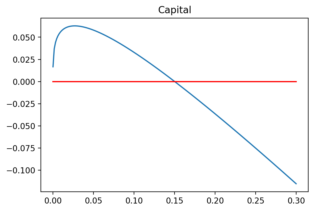
From the graph we see that optimal capital is roughly around 0.15. We next use the fsolve root finding algorithm from the scipy.optimize library. Go back to the chapter on root finding and review the various root finding algorithms such as Newton-Raphson, Secant Method, Bracketing as well as the built in root and fsolve.
from scipy.optimize import fsolve

# Use built in 'fsolve'
print(" ")
print(" -------------- Fsolve ------------")

k_guess = 2  # our starting guess
solutionK = fsolve(func, k_guess) # starting from K = 2

# Kstar is a numpy array which does not print well
# We therefore change it into a 'pure' number
# so we can use the print format to create a nice
# looking output
Kstar = solutionK[0]

Ystar = A*Kstar**alpha*L**(1-alpha)
qstar = alpha*A*Kstar**(alpha-1)
rstar = qstar - delta
Rstar = 1. + (1-tau_K)*(qstar - delta)
wstar = (1.-alpha)*A*Kstar**alpha

# Back out solutions for the rest of the Economy
# ----------------------------------------------
# Household values
sstar = Kstar/N_y
cystar= (1.-tau_L)*wstar + t_y - sstar
costar= Rstar*sstar + t_o

# Residual gov't consumption, thrown in the ocean
Gstar = N_y*tau_L*wstar + N_o*tau_K*rstar*sstar

# Aggregate consumption
Cstar = N_y*cystar + N_o*costar

# Check the goods market condition or Aggregate resource constraint
ARC = Ystar - delta*Kstar - Cstar - Gstar

# Print results
print(" -------------------------------------")
print(" Root finding ")
print(" -------------------------------------")
print("K* = {:6.4f}".format(Kstar))
print("Y* = {:6.4f}".format(Ystar))
print("q* = {:6.4f}".format(qstar))
print("r* = {:6.4f}".format(rstar))
print("R* = {:6.4f}".format(Rstar))
print("w* = {:6.4f}".format(wstar))
print(" -------------------------------------")
print("ARC = {:6.4f}".format(ARC))
 -------------- Fsolve ------------
 -------------------------------------
 Root finding
 -------------------------------------
K* = 0.1502
Y* = 0.5662
q* = 1.1310
r* = 1.1310
R* = 1.9613
w* = 0.3964
 -------------------------------------
ARC = 0.0000
21.5. Method 2: Gauss-Seidl Algorithm
Instead of substituting and solving for one equation in one unknown we can use the so called Gauss-Seidl method.
It is an iterative method where we guess a starting value for capital. We then use this starting guess as if it was a solution to the model and back out all the other endogenous variables.
We then use these “solutions” of endogenous variables and calculate the new capital that would be the result of household savings and consumption decisions.
We then update our first guess of capital K, with this new and better guess and do it all over again.
We repeat this until the guess of capital at the beginning of the algorithm is roughly the same as the calculated capital at the end of the algorithm. This is a referred to as a fixed point (once Knew = Kold).
Here is the algorithm in more detail:
Note
Gauss-Seidl Algorithm
- Step 1.
For this method we start with a guess for capital \(K_{old}\)
- Step 2.
We then solve for prices \(w,R,q\)
\[w = (1-\alpha)*K_{old}^{\alpha} \times L^{-\alpha}\]\[q = \alpha \times A \times K_{old}^{(\alpha-1)} \times L^{1-\alpha}\]\[R = 1 + (1-\tau_K)(q - \delta)\]- Step 3.
We then solve for optimal household savings \(s^*\)
\[s^* = N_y \frac{\beta R ((1-\tau_L)w + t_y) - t_o}{(1+\beta)R}\]- Step 4.
We then aggregate over all households and get the new capital stock \(K_{new}\)
\[K_{new}=N_y \times s^*\]- Step 5.
Calculate error and check whether algorithm has converged
\[\text{error} = (K_{old} - K_{new})/K_{old}\]- Step 6.
We then update capital \(K_{old} = \lambda * K_{new} + (1-\lambda) * K_{old}\) and repeat from Step 2 above. Note that \(0 < \lambda < 1\) is an updating parameter.
Python Program 2
# Guess capital stock
glamda  = 0.5   # updating parameter
Kold    = 0.4
jerror  = 100
iter    = 1
while (iter<200) or (jerror>0.001):
    # Solve for prices using expressions for w(K) and q(K)
    q = alpha*A*Kold**(alpha-1)
    w = (1-alpha)*A*Kold**alpha
    R = 1 + (1-tau_K)*(q - delta)
    Knew = N_y* (beta*R*((1-tau_L)*w + t_y) - t_o)/((1+beta)*R)
    # Calculate discrepancy between old and new capital stock
    jerror = abs(Kold-Knew)/Kold
    # Update capital stock
    Kold    = glamda*Knew + (1-glamda)*Kold
    iter = iter +1

# Print results
Kstar = Knew
Ystar = A*Kstar**alpha*L**(1-alpha)
wstar = w
qstar = q
Rstar = R
rstar = qstar - delta

# ------------------------------------
# Back out solutions for the rest of the Economy

# Household values
sstar = Kstar/N_y
cystar= (1-tau_L)*wstar + t_y - sstar
costar= Rstar*sstar + t_o

# Residual gov't consumption, thrown in the ocean
Gstar = N_y*tau_L*wstar + N_o*tau_K*rstar*sstar

# Aggregate consumption
Cstar = N_y*cystar + N_o*costar

# Check the goods market condition or Aggregate resource constraint
ARC = Ystar - delta*Kstar - Cstar - Gstar

print(" -------------------------------------")
print(" Gauss-Seidl ")
print(" -------------------------------------")
print("Nr. of iterations = " +str(iter))
print("K* = {:6.4f}".format(Kstar))
print("Y* = {:6.4f}".format(Ystar))
print("q* = {:6.4f}".format(qstar))
print("r* = {:6.4f}".format(rstar))
print("R* = {:6.4f}".format(Rstar))
print("w* = {:6.4f}".format(wstar))
print(" -------------------------------------")
print("ARC = {:6.4f}".format(ARC))
 -------------------------------------
 Gauss-Seidl
 -------------------------------------
Nr. of iterations = 200
K* = 0.1502
Y* = 0.5662
q* = 1.1310
r* = 1.1310
R* = 1.9613
w* = 0.3964
 -------------------------------------
ARC = 0.0000
21.6. Tax Policy Simulation
Now that we have solved the model for an equilibrium we can use this model to conduct policy simulations such as a tax policy reform. When we first solved this model the tax on labor was \(\tau_L = 20\%\). What would happen if the government were to raise the labor tax to \(\tau_L = 25\%\)?
Well, just plug it in and resolve the model. Then compare the prior GDP (i.e. variable Y) to the new GDP.
What has happened?
Make before and after graphs (maybe a bar chart that shows Y, C, K before and after the tax increase) and discuss your results.
Python Program 3: Gauss-Seidl after tax increase from 20 to 25%
# Set new parameter values
N_y     = 1.0
N_o     = 1.0
alpha   = 0.3
A       = 1
beta    = 0.9
delta   = 0.0
tau_L   = 0.25  #Old value: tau_L   = 0.2
tau_K   = 0.15
t_y     = 0.0
t_o     = 0.0
#
L       = 1

# Guess capital stock
glamda  = 0.5   # updating parameter
Kold    = 0.4
jerror  = 100
iter    = 1
while (iter<200) or (jerror>0.001):
    # Solve for prices using expressions for w(K) and q(K)
    q = alpha*A*Kold**(alpha-1)
    w = (1-alpha)*A*Kold**alpha
    R = 1 + (1-tau_K)*(q - delta)
    Knew = N_y* (beta*R*((1-tau_L)*w + t_y) - t_o)/((1+beta)*R)
    # Calculate discrepancy between old and new capital stock
    jerror = abs(Kold-Knew)/Kold
    # Update capital stock
    Kold    = glamda*Knew + (1-glamda)*Kold
    iter = iter +1

# Print results
Kstar_new = Knew
Ystar_new  = A*Kstar_new**alpha*L**(1-alpha)
wstar_new  = w
qstar_new  = q
Rstar_new  = R
rstar_new  = q - delta

# ------------------------------------
# Back out solutions for the rest of the Economy

# Household values
sstar_new = Kstar_new/N_y
cystar_new= (1-tau_L)*wstar_new + t_y - sstar_new
costar_new= Rstar_new*sstar_new + t_o

# Residual gov't consumption, thrown in the ocean
Gstar_new = N_y*tau_L*wstar_new + N_o*tau_K*rstar_new*sstar_new

# Aggregate consumption
Cstar_new = N_y*cystar_new + N_o*costar_new

# Check the goods market condition or Aggregate resource constraint
ARC_new = Ystar_new - delta*Kstar_new - Cstar_new - Gstar_new

print(" -------------------------------------")
print(" Gauss-Seidl: tau_L = 25% ")
print(" -------------------------------------")
print("Nr. of iterations = " +str(iter))
print("K* = {:6.4f}".format(Kstar_new))
print("Y* = {:6.4f}".format(Ystar_new))
print("q* = {:6.4f}".format(qstar_new))
print("r* = {:6.4f}".format(rstar_new))
print("R* = {:6.4f}".format(Rstar_new))
print("w* = {:6.4f}".format(wstar_new))
print(" -------------------------------------")
print("ARC = {:6.4f}".format(ARC_new))
 -------------------------------------
 Gauss-Seidl: tau_L = 25%
 -------------------------------------
Nr. of iterations = 200
K* = 0.1370
Y* = 0.5508
q* = 1.2063
r* = 1.2063
R* = 2.0254
w* = 0.3856
 -------------------------------------
ARC = 0.0000
Discuss results.
print(" -------------------------------------")
print(" Gauss-Seidl: tau_L = 20% ")
print(" -------------------------------------")
print("K* = {:6.4f}".format(Kstar))
print("Y* = {:6.4f}".format(Ystar))
print("q* = {:6.4f}".format(qstar))
print("r* = {:6.4f}".format(rstar))
print("R* = {:6.4f}".format(Rstar))
print("w* = {:6.4f}".format(wstar))

print(" -------------------------------------")
print(" Gauss-Seidl: tau_L = 25% ")
print(" -------------------------------------")
print("K* = {:6.4f}".format(Kstar_new))
print("Y* = {:6.4f}".format(Ystar_new))
print("q* = {:6.4f}".format(qstar_new))
print("r* = {:6.4f}".format(rstar_new))
print("R* = {:6.4f}".format(Rstar_new))
print("w* = {:6.4f}".format(wstar_new))
print(" -------------------------------------")
 -------------------------------------
 Gauss-Seidl: tau_L = 20%
 -------------------------------------
K* = 0.1502
Y* = 0.5662
q* = 1.1310
r* = 1.1310
R* = 1.9613
w* = 0.3964
 -------------------------------------
 Gauss-Seidl: tau_L = 25%
 -------------------------------------
K* = 0.1370
Y* = 0.5508
q* = 1.2063
r* = 1.2063
R* = 2.0254
w* = 0.3856
 -------------------------------------
21.7. Key Concepts and Summary
Note
Introduction of OLG model
Deriving optimality conditions in OLG model
Introduction of non-linear function solution
Gauss-Seidl Algorithm
21.8. Self-Check Questions
Todo
Use either one of the models above and resolve the model for \(\tau_K = [0.01, 0.02, 0.03,...,0.1]\) and track output, agggregate capital and tax revenue from capital as well as labor taxes.
Repeat the exercise above but this time change the labor tax parameter and resolve the model for \(\tau_L = [0.11, 0.12, 0.13,...,0.2]\)