11. Working with Data II: Statistics
In this chapter we introduce summary statistics and statistical graphing
methods using the pandas and the statsmodels library.
11.1. Importing Data
We will be working with three data sets.
Lecture_Data_Excel_a.csv.
Lecture_Data_Excel_b.csv.
Lecture_Data_Excel_c.xlsx.
import numpy as np
import matplotlib.pyplot as plt
import pandas as pd
import statsmodels.api as sm
#from ggplot import *
from scipy import stats as st
import math as m
import seaborn as sns
import time  # Imports system time module to time your script

plt.close('all')  # close all open figures
# Read in small data from .csv file
# Filepath
filepath = 'Lecture_Data/'
# In windows you can also specify the absolute path to your data file
# filepath = 'C:/Dropbox/Towson/Teaching/3_ComputationalEconomics/Lectures/Lecture_Data/'

# ------------- Load data --------------------
df = pd.read_csv(filepath + 'Lecture_Data_Excel_a.csv', dtype={'Frequency': float})

df = df.drop('Unnamed: 2', axis=1)
df = df.drop('Unnamed: 3', axis=1)
Let us now have a look at the dataframe to see what we have got.
print(df)
                 Area  Frequency
0          Accounting       73.0
1             Finance       52.0
2  General management       36.0
3     Marketing sales       64.0
4               other       28.0
We have data on field of study in the column Area and we have absolute
frequences that tell us how many students study in those areas. We next form
relative frequencies by dividing the absolute frequencies by the total number
of students. We put the results in a new column called relFrequency.
# Make new column with relative frequency
df['relFrequency'] = df['Frequency']/df['Frequency'].sum()
# Let's have a look at it, it's a nested list
print(df)
                 Area  Frequency  relFrequency
0          Accounting       73.0      0.288538
1             Finance       52.0      0.205534
2  General management       36.0      0.142292
3     Marketing sales       64.0      0.252964
4               other       28.0      0.110672
We can now interact with the DataFrame. Let us first simply “grab” the relative frequencies out of the DataFrame into a numpy array. This is now simply a numerical vector that you have already worked with in previous chapters.
xv = df['relFrequency'].values
print('Array xv is:', xv)
Array xv is: [0.28853755 0.2055336 0.14229249 0.25296443 0.11067194]
11.2. Making Simple Graphs from our Data
11.2.1. Bar Charts
We first make a bar chart of the absolute frequencies.
fig, ax = plt.subplots()

ax.plot(1. + np.arange(len(xv)), xv, '-o')
plt.show()
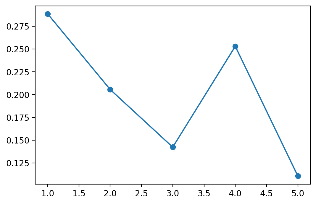
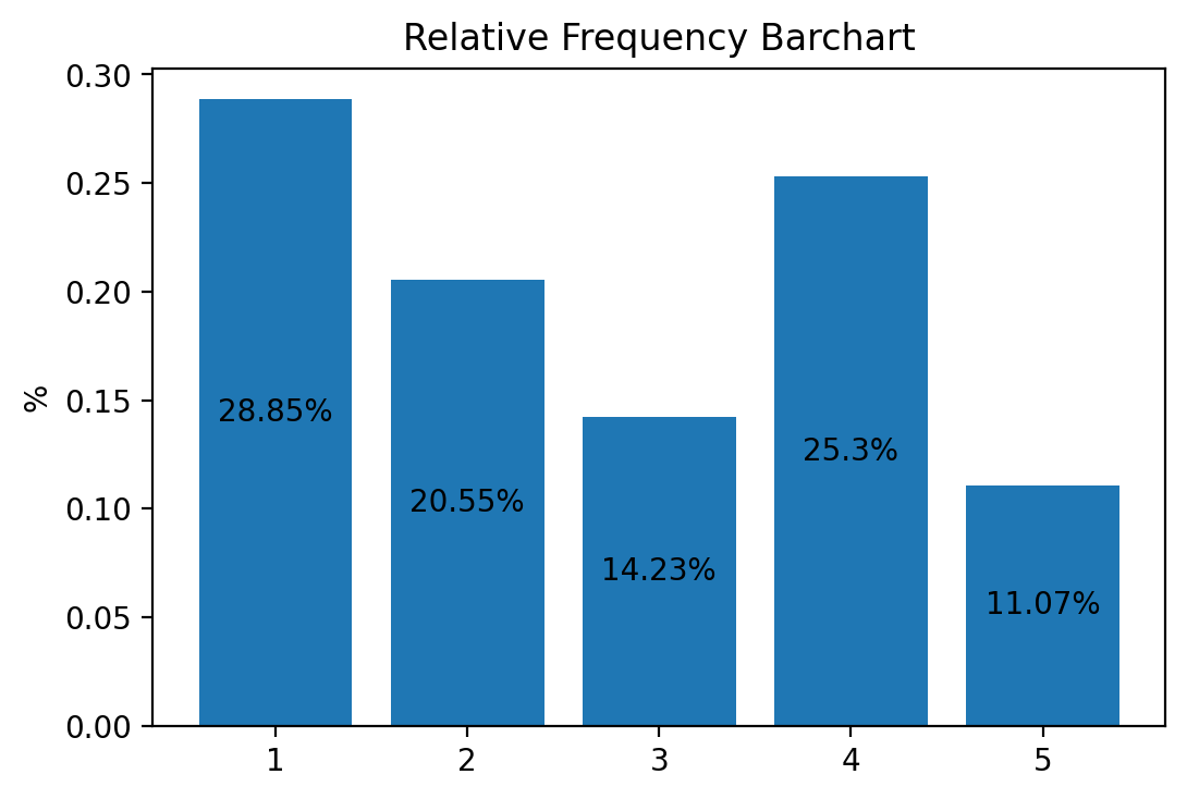
Hey, that’s not a bar chart. Let’s try again.
fig, ax = plt.subplots()

ax.bar(1. + np.arange(len(xv)), xv, align='center')

# Annotate with text
ax.set_xticks(1. + np.arange(len(xv)))
for i, val in enumerate(xv):
    ax.text(i+1, val/2, str(round(val*100, 2))+'%', va='center', ha='center', color='black')
ax.set_ylabel('%')
ax.set_title('Relative Frequency Barchart')
plt.show()

# We can also save this graph as a pdf in a subfolder called 'Graphs'
# You will have to make this subfolder first though.

#savefig('./Graphs/fig1.pdf')
This simple command plots the barchart into a window and saves it as
fig1.pdf into a subfolder called Graphs. Don’t forget to first make
this subfolder, otherwise Python will throw an error when it can’t find the
folder.
You also see that the height of the bars is symply the y-coordinate of the points in the previous scatter plot.
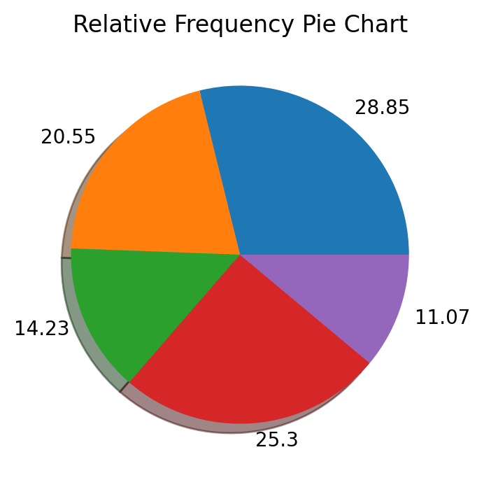
11.2.2. Pie Charts
We next make a pie chart using the relative frequencies stored in vector xv.
fig, ax = plt.subplots()
ax.pie(xv, labels = np.round(xv*100, 2), shadow=True)
# Annotate with text
ax.set_title('Relative Frequency Pie Chart')
plt.show()
11.2.3. Histograms
Next we use a new data file called
Lecture_Data_Excel_b.csv.
Let us first import the data and have a quick look.
df = pd.read_csv(filepath + 'Lecture_Data_Excel_b.csv')
print(df.head())
   Height  Response  AverageMathSAT  Age  Female  Education  Race
0     1.1         3             370   20       0          2  Hisp
1     1.2         4             393   20       0          4   Wht
2     1.3         4             413   20       0          4   Blk
3     1.4         5             430   20       0          4   Wht
4     1.5         3             440   20       0          2   Mex
Let us clean this somewhat and drop a column
that we do not plan on using, the Response column.
df = pd.read_csv(filepath + 'Lecture_Data_Excel_b.csv')
df = df.drop('Response' , axis=1)
print(df.head())
   Height  AverageMathSAT  Age  Female  Education  Race
0     1.1             370   20       0          2  Hisp
1     1.2             393   20       0          4   Wht
2     1.3             413   20       0          4   Blk
3     1.4             430   20       0          4   Wht
4     1.5             440   20       0          2   Mex
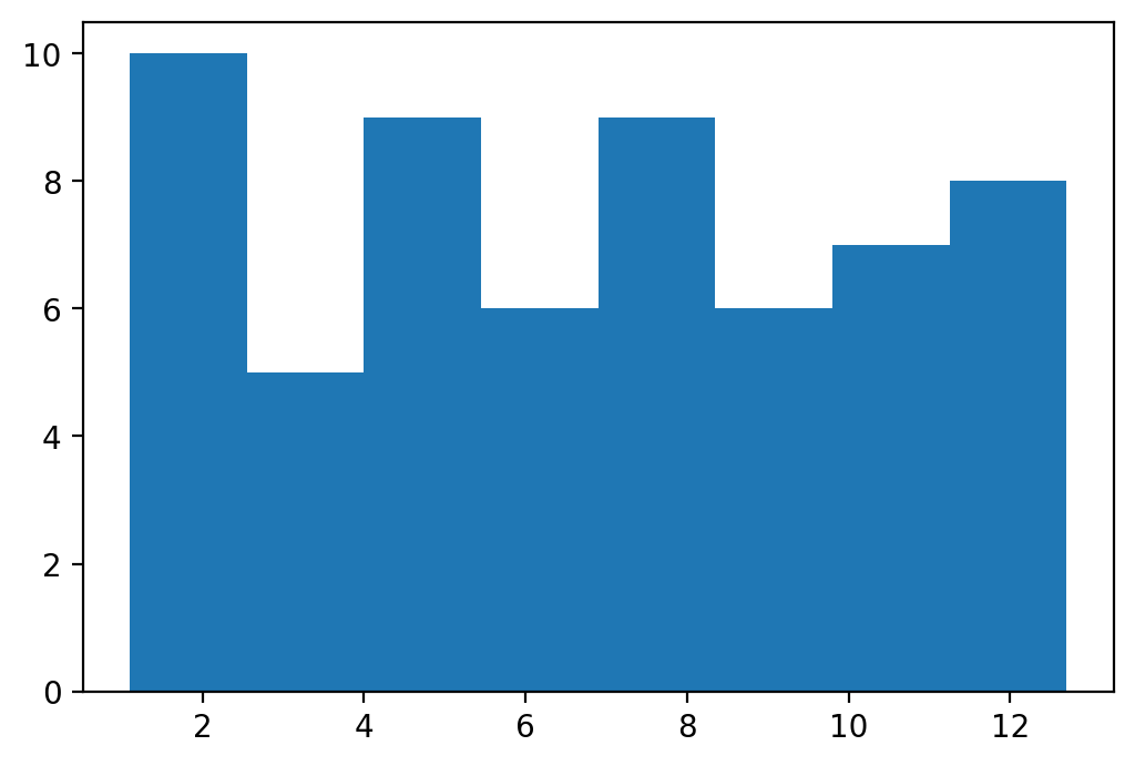
The remaining data in the DataFrame has observations on on height, age and
other variables. We first make a histogram of the continuous variable Height.
The actual command for the histogram is hist. It returns three variables
prob, bins, and patches. We use them in the following to add
information to the histogram.
heightv = df['Height'].values

# Initialize
N = len(heightv) # number of obs.
B = 8           # number of bins in histogram

fig, ax = plt.subplots()
plt.subplots_adjust(wspace = 0.8, hspace = 0.8)

prob, bins, patches = ax.hist(heightv, bins=B, align='mid' )
plt.show()
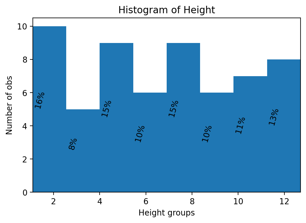
We next add some text to the histogram so that we can convey even more information to the reader/user of our research.
heightv = df['Height'].values

# Initialize
N = len(heightv) # number of obs.
B = 8           # number of bins in histogram

fig, ax = plt.subplots()
plt.subplots_adjust(wspace = 0.8, hspace = 0.8)

prob, bins, patches = ax.hist(heightv, bins=B, align='mid' )
# Annotate with text
for i, p in enumerate(prob):
    percent = int(float(p)/N*100)
    # only annotate non-zero values
    if percent:
        ax.text(bins[i]+0.3, p/2.0, str(percent)+'%', rotation=75, va='bottom', ha='center')

ax.set_xlabel('Height groups')
ax.set_ylabel('Number of obs')
ax.set_title('Histogram of Height')
ax.set_xlim(min(heightv),max(heightv))

plt.show()
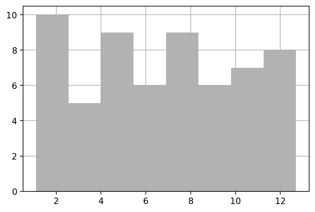
We can also make histograms with pandas built in commands. However, with
this method you have less information about where the bars appear and what
height they are, so you won’t be able to add text at the appropriate positions
as conveniently as before.
heightv = df['Height'].values

# Initialize
N = len(heightv) # number of obs.
B = 8           # number of bins in histogram

fig, ax = plt.subplots()
plt.subplots_adjust(wspace = 0.8, hspace = 0.8)

df['Height'].hist(bins = B, ax = ax, color = 'k', alpha = 0.3)
#
plt.show()
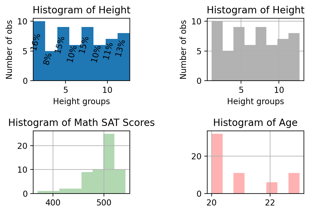
Now we add a couple more variables and make a series of histograms all in the same figure.
heightv = df['Height'].values

# Initialize
N = len(heightv) # number of obs.
B = 8           # number of bins in histogram

fig, ax = plt.subplots(2,2)
plt.subplots_adjust(wspace = 0.8, hspace = 0.8)

prob, bins, patches = ax[0,0].hist(heightv, bins=B, align='mid' )
# Annotate with text
for i, p in enumerate(prob):
    percent = int(float(p)/N*100)
    # only annotate non-zero values
    if percent:
        ax[0,0].text(bins[i]+0.3, p/2.0, str(percent)+'%', rotation=75, va='bottom', ha='center')

ax[0,0].set_xlabel('Height groups')
ax[0,0].set_ylabel('Number of obs')
ax[0,0].set_title('Histogram of Height')
ax[0,0].set_xlim(min(heightv),max(heightv))

# Using Panda's built in histogram method
df['Height'].hist(bins = B, ax = ax[0,1], color = 'k', alpha = 0.3)
ax[0,1].set_title('Histogram of Height')
ax[0,1].set_xlabel('Height groups')
ax[0,1].set_ylabel('Number of obs')
#
df['AverageMathSAT'].hist(bins = B, ax = ax[1,0], color = 'g', alpha = 0.3)
ax[1,0].set_title('Histogram of Math SAT Scores')
#
#
df['Age'].hist(bins = B, ax = ax[1,1], color = 'r', alpha = 0.3)
ax[1,1].set_title('Histogram of Age')
#
plt.show()
Note
Another way to graph a histogram is by using the powerful ggplot package
which is a translation of R’s ggplot2 package into Python. It
follows a completely different graphing philosophy based on the grammar of
grapics by:
Hadley Wickham. A layered grammar of graphics. Journal of Computational and Graphical Statistics, vol. 19, no. 1, pp. 3–28, 2010.
After installing the ggplot library, you would plot the data as follows:
print( ggplot(aes(x='Height'), data = df) + geom_histogram() +
ggtitle("Histogram of Height using ggplot") + labs("Height", "Freq"))
Warning
The ggplot Python version seems to not be compatible with the
latest version of Python 3.6. You would need to install an older version of
Python if you wanted to use this library as of writing this.
We can also use the seaborn library to make fancy looking histograms
quickly as in Histogram2.
import seaborn as sns
sns.histplot(df['AverageMathSAT'].dropna(),bins=10, color='g')
plt.show()
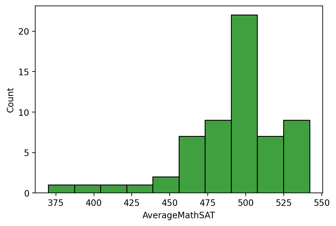
Fig. 11.1 Histogram with Distribution Added
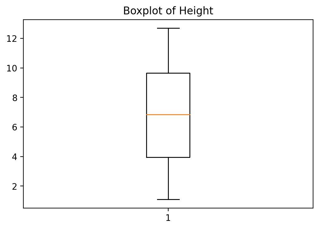
11.2.4. Boxplots
A boxplot of height is made as follows:
fig, ax = plt.subplots()
ax.boxplot(heightv)
# Annotate with text
ax.set_title('Boxplot of Height')
plt.show()
11.3. Summary Statistics
We next go through some basic summary statistics measures.
11.3.1. Measures of Central Tendency
A quick way to produce summary statistics of our data set is to use panda's
command describe.
print(df.describe())
          Height  AverageMathSAT        Age     Female  Education
count  60.000000       60.000000  60.000000  60.000000  60.000000
mean    6.816667      493.666667  20.933333   0.333333   3.016667
std     3.571743       34.018274   1.176992   0.475383   1.096863
min     1.100000      370.000000  20.000000   0.000000   1.000000
25%     3.950000      478.500000  20.000000   0.000000   2.000000
50%     6.850000      507.000000  20.000000   0.000000   3.000000
75%     9.650000      509.250000  22.000000   1.000000   4.000000
max    12.700000      542.000000  23.000000   1.000000   5.000000
Or we can produce the same statistics by hand. We first calculate the mean,
median and mode. Note that mode is part of the stats package which was
imported as st using: from scipy import stats as st. Now we have to add
st to the mode command: st.mode(heightv) in order to call it. The other
commands are part of the numpy package so they have the prefix np.
# Number of observations (sample size)
N = len(heightv)

# Mean - Median - Mode
print("Mean(height)=  {:.3f}".format(np.mean(heightv)))
print("Median(height)=  {:.3f}".format(np.median(heightv)))

# Mode (value with highest frequency)
print("Mode(height)=  {}".format(st.mode(heightv)))
Mean(height)=  6.817
Median(height)=  6.850
Mode(height)=  ModeResult(mode=array([1.1]), count=array([1]))
We can also just summarize a variable using the st.describe command from
the stats package.
# Summary stats
print("Summary Stats")
print("-------------")
print(st.describe(heightv))
Summary Stats
-------------
DescribeResult(nobs=60, minmax=(1.1, 12.7), mean=6.8166666666666655,
variance=12.757344632768362, skewness=0.019099619781273072,
kurtosis=-1.1611486008105545)
11.3.2. Measures of Dispersion
We now calculate the range, variance and standard deviations. Remember that for variance and standard deviation there is a distinction between population and sample.
# returns smallest a largest element
print("Range = {:.3f}".format(max(heightv)-min(heightv)))
print("Population variance = {:.3f}".\

# population variance
  format(np.sum((heightv-np.mean(heightv))**2)/N))

# sample variance
print("Sample variance     = {:.3f}".\
  format(np.sum((heightv-np.mean(heightv))**2)/(N-1)))

print("Pop.   standard dev = {:.3f}".\
  format(np.sqrt(np.sum((heightv-np.mean(heightv))**2)/N)))

print("Sample standard dev = {:.3f}". \
  format(np.sqrt(np.sum((heightv-np.mean(heightv))**2)/(N-1))))

#Or simply
print("Pop.   standard dev = {:.3f}".format(np.std(heightv)))
Range = 11.600
Population variance = 12.545
Sample variance     = 12.757
Pop.   standard dev = 3.542
Sample standard dev = 3.572
Pop.   standard dev = 3.542
11.3.3. Measures of Relative Standing
Percentiles are calculated as follows:
print("1 quartile (25th percentile) = {:.3f}".\
  format(st.scoreatpercentile(heightv, 25)))
print("2 quartile (50th percentile) = {:.3f}".\
  format(st.scoreatpercentile(heightv, 50)))
print("3 quartile (75th percentile) = {:.3f}".\
  format(st.scoreatpercentile(heightv, 75)))

# Inter quartile rante: Q3-Q1 or P_75-P_25
print("IQR = P75 - P25              = {:.3f}".\
  format(st.scoreatpercentile(heightv, 75)\
  -st.scoreatpercentile(heightv, 25)))
1 quartile (25th percentile) = 3.950
2 quartile (50th percentile) = 6.850
3 quartile (75th percentile) = 9.650
IQR = P75 - P25              = 5.700
11.3.4. Data Aggregation or Summary Statistics by Subgroup
We next want to summarize the data by subgroup. Let’s assume that we would like
to compare the average Height by Race. We can use the groupby() to
accomplish this.
groupRace = df.groupby('Race')
print('Summary by Race', groupRace.mean())
Summary by Race         Height  AverageMathSAT        Age    Female
Education
Race
Blk   6.278261      491.652174  20.826087  0.304348   3.565217
Hisp  6.525000      472.750000  21.500000  0.250000   1.750000
Mex   6.171429      491.571429  20.928571  0.285714   2.428571
Oth   8.750000      516.000000  21.000000  0.500000   2.500000
Wht   7.917647      500.411765  20.941176  0.411765   3.117647
We could also use a different category like gender.
groupGender = df.groupby('Female')
print('Summary by Gender', groupGender.mean())
Summary by Gender         Height  AverageMathSAT   Age  Education
Female
0        4.765           479.7  21.4       2.95
1       10.920           521.6  20.0       3.15
Or we can also combine the two or more categories and summarize the data as follows.
groupRaceGender = df.groupby(['Race', 'Female'])
print('Summary by Race and Gender', groupRaceGender.mean())
Summary by Race and Gender                 Height  AverageMathSAT
Age  Education
Race Female
Blk  0        4.350000      479.562500  21.1875   3.562500
     1       10.685714      519.285714  20.0000   3.571429
Hisp 0        5.600000      461.333333  22.0000   1.666667
     1        9.300000      507.000000  20.0000   2.000000
Mex  0        4.480000      481.900000  21.3000   2.100000
     1       10.400000      515.750000  20.0000   3.250000
Oth  0        6.300000      506.000000  22.0000   1.000000
     1       11.200000      526.000000  20.0000   4.000000
Wht  0        5.310000      480.600000  21.6000   3.400000
     1       11.642857      528.714286  20.0000   2.714286
Be careful and don’t forget to add the various categories in a list using the
brackets [...]].
11.4. Measures of Linear Relationship
11.4.1. Covariance
We first grab two variables heightv and agev from the dataframe and
define them as numpy arrays.
xv = df['Age'].values
yv = df['Height'].values
n = len(xv)
We then go ahead and calculate the covariance.
# Population covariance
print("Population covariance = {:.3f}".\
  format(np.sum((xv-np.mean(xv))*(yv-np.mean(yv)))/n))

# Sample covariance
print("Sample covariance     = {:.3f}".\
  format(np.sum((xv-np.mean(xv))*(yv-np.mean(yv)))/(n-1)))

# or simply
print("Sample covariance     = {:.3f}".format(df.Age.cov(df.Height)))
Population covariance = -0.159
Sample covariance     = -0.162
Sample covariance     = -0.162
11.4.2. Correlation Coefficient
We can calculate the correlation coefficient by hand or using the pandas
toolbox command.
print("Correlation coefficient =  {:.3f}".\
  format((np.sum((xv-np.mean(xv))*(yv-np.mean(yv)))/n)\
  /(np.std(xv)*np.std(yv))))

print("Correlation coefficient = {:.3f}".format(df.Age.corr(df.Height)))
Correlation coefficient =  -0.038
Correlation coefficient = -0.038
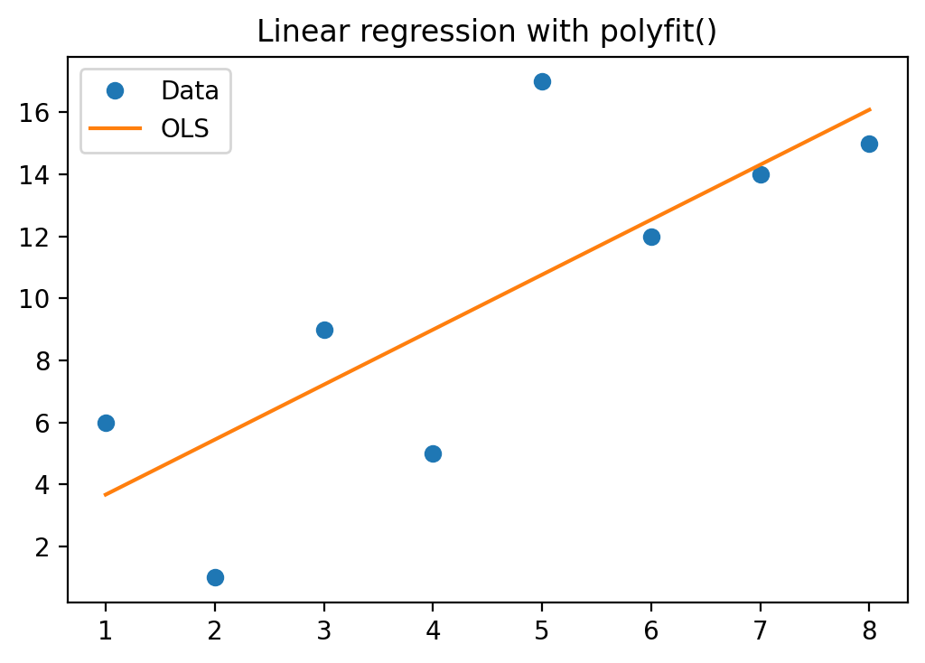
11.4.3. Regression Line: Example 1
We first generate some data. A variable x and a variable y.
# Define data. 2 vectors xv and yv
xv = np.arange(1,9,1)
yv = np.array([6,1,9,5,17,12,14,15])
We then “cast” these into a pandas DataFrame.
# Define data frame
df = pd.DataFrame(np.array([xv, yv]).T, columns = ['x', 'y'])
We fist make a scatterplot with least squares trend line: y = beta_0 + beta_1 * x + epsilon.
p = np.polyfit(xv, yv, 1)
print("p = {}".format(p))

# Scatterplot
fig, ax = plt.subplots()
ax.set_title('Linear regression with polyfit()')
ax.plot(xv, yv, 'o', label = 'data')
ax.plot(xv, np.polyval(p,xv),'-', label = 'Linear regression')
ax.legend(['Data', 'OLS'], loc='best')
plt.show()
p = [1.77380952 1.89285714]
Example 1 Again with Statsmodels library
We then run the same regression using a more general method called ols
which is part of statsmodels. When calling the ols function
you need to add the module name (statsmodels was imported as sm)
in front of it: sm.OLS(). You then define the independent variable y
and the dependent variables x's.
Warning
If you google for OLS and Python you may come across code that
uses Pandas directly to run an OLS regression as in pd.OLS(y=Ydata,
x=Xdata). This will not work anymore as this API has been deprecated in
newer versions of Pandas. You need to use the
Statsmodel Library
import statsmodels.api as sm
from patsy import dmatrices

# Run OLS regression
# This line adds a constant number column to the X-matrix and extracts
# the relevant columns from the dataframe
y, X = dmatrices('y ~ x', data=df, return_type='dataframe')
res = sm.OLS(y, X).fit()

# Show coefficient estimates
print(res.summary())
                            OLS Regression Results
==============================================================================
Dep. Variable:                      y   R-squared:
0.609
Model:                            OLS   Adj. R-squared:
0.544
Method:                 Least Squares   F-statistic:
9.358
Date:                Thu, 12 May 2022   Prob (F-statistic):
0.0222
Time:                        15:51:22   Log-Likelihood:
-20.791
No. Observations:                   8   AIC:
45.58
Df Residuals:                       6   BIC:
45.74
Df Model:                           1
Covariance Type:            nonrobust
==============================================================================
                 coef    std err          t      P>|t|      [0.025
0.975]
------------------------------------------------------------------------------
Intercept      1.8929      2.928      0.646      0.542      -5.272
9.058
x              1.7738      0.580      3.059      0.022       0.355
3.193
==============================================================================
Omnibus:                        0.555   Durbin-Watson:
3.176
Prob(Omnibus):                  0.758   Jarque-Bera (JB):
0.309
Skew:                           0.394   Prob(JB):
0.857
Kurtosis:                       2.449   Cond. No.
11.5
==============================================================================

Notes:
[1] Standard Errors assume that the covariance matrix of the errors is
correctly specified.
/home/jjung/anaconda3/envs/pweaveEnv/lib/python3.9/site-
packages/scipy/stats/stats.py:1541: UserWarning: kurtosistest only
valid for n>=20 ... continuing anyway, n=8
  warnings.warn("kurtosistest only valid for n>=20 ... continuing "
Or if you simply want to have a look at the estimated coefficients you can access them via:
print('Parameters:')
print(res.params)
Parameters:
Intercept    1.892857
x            1.773810
dtype: float64
Finally, we use the model to make a prediction of y when x = 8.5.
# Make prediction for x = 8.5
betas = res.params.values
print("Prediction of y for x = 8.5 is: {:.3f}".\
  format(np.sum(betas * np.array([1,8.5]))))
Prediction of y for x = 8.5 is: 16.970
We can also use the results from the OLS command to make a scatterplot with
the trendline through it.
fig, ax = plt.subplots()
ax.set_title('Linear Regression with Fitted Values')
ax.plot(xv, yv, 'o', label = 'data')
ax.plot(xv, res.predict(X).values,'k-', label = 'Linear regression')
ax.legend(['Data', 'OLS'], loc='best')
plt.show()
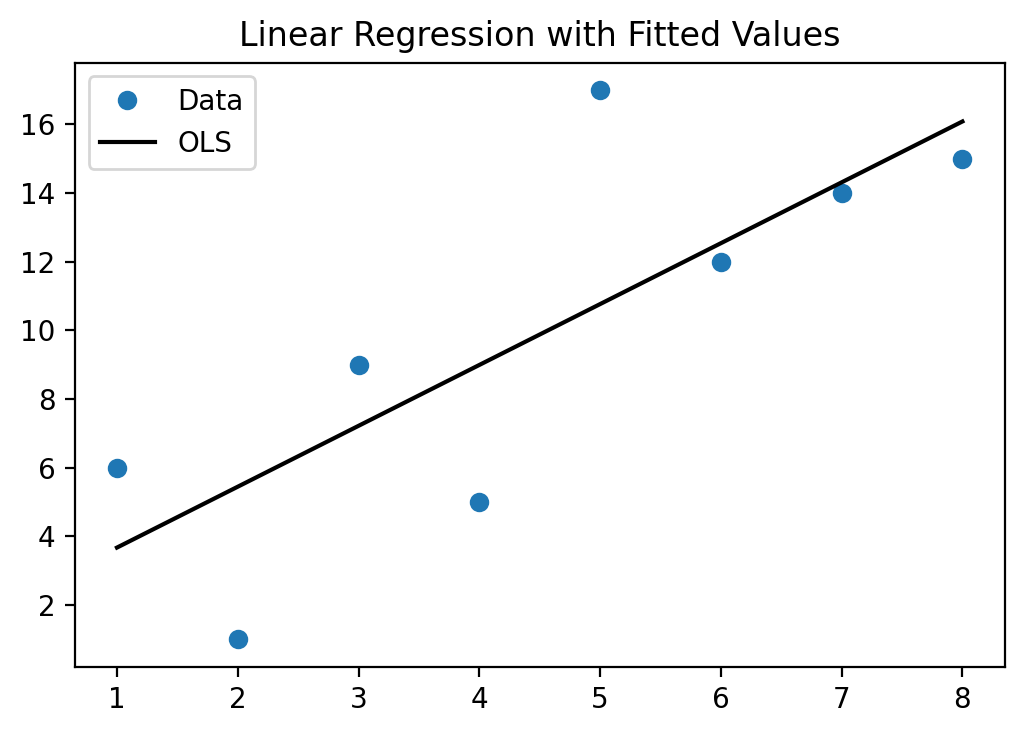
As you have seen above, you can use the estimates from this model to make predictions of Y (called Y-hat) for specific values of variable X. We next use all the X values from our original data and predict for each one of those what the corresponding predicted Y-value would be (\(\hat{y}\)) and then calculate the difference between the actual Y value in the data and the predicted Y-value Y-hat. In the graph above, it is essentially the distance of the blue dots (the data) to the black line (the prediction from the model). These differences, \(y-\hat{y}\), are also called the residual errors of your model. The OLS procedure tries to find beta estimates to minimize these residual errors (OLS actually tried to minimize the sum of all the squared errors, or \(\sum_i{(y_i-\hat{y}_i)^2}\).
Here is the code to accomplish this.
y_hatv = res.predict(X).values  # Predicts y-hat based on all X values in data
residualsv = yv - y_hatv

fig, ax = plt.subplots()
ax.set_title('Residual Plot')
ax.plot(yv, residualsv, 'o', label = 'data')
ax.plot(yv, np.zeros(len(yv)),'k-')
ax.set_xlabel('Y - Dependent Variable')
plt.show()
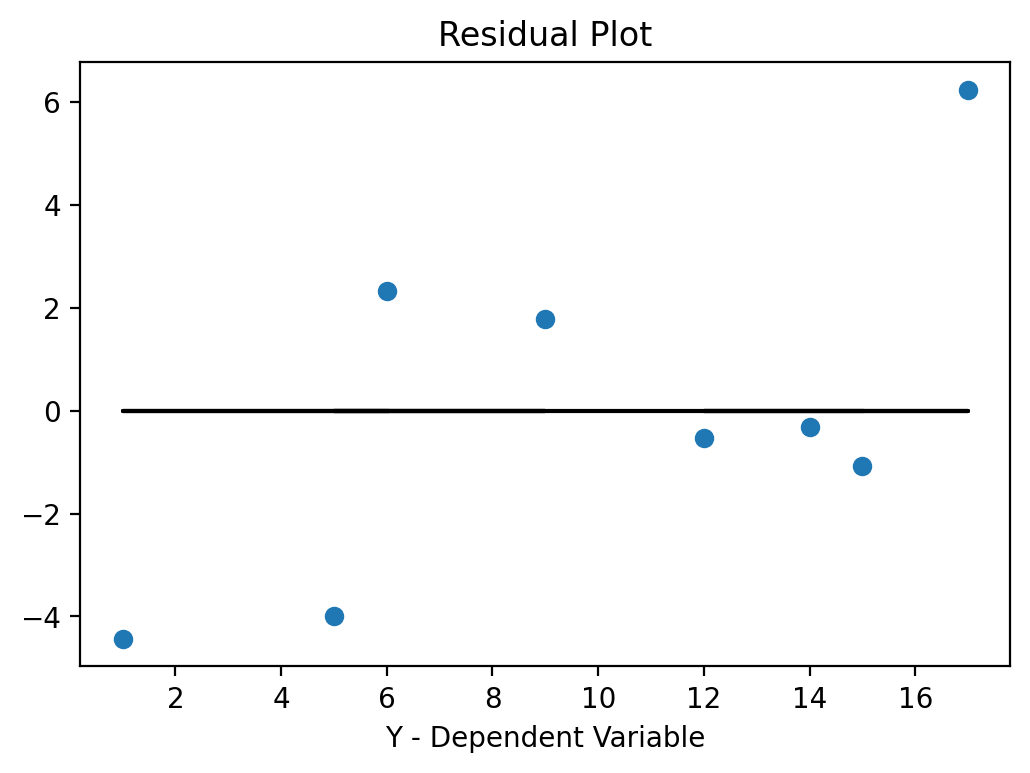
If the errors are systematically different over the range of X-values we call this heteroskedasticity. If you dedect heteroskedasticity you would have to adjust for that using a more “robust” estimator. These more robust procedures basically adjust the standard errors (make them larger) to account for the effect that heteroskedasticity has on your estimate.
Here is how you estimate the “robust” version of your regression.
import statsmodels.api as sm
from patsy import dmatrices

# Run OLS regression
# This line adds a constant number column to the X-matrix and extracts
# the relevant columns from the dataframe
y, X = dmatrices('y ~ x', data=df, return_type='dataframe')
res_rob = sm.OLS(y, X).fit(cov_type = 'HC3')

# Show coefficient estimates
print(res_rob.summary())
                            OLS Regression Results
==============================================================================
Dep. Variable:                      y   R-squared:
0.609
Model:                            OLS   Adj. R-squared:
0.544
Method:                 Least Squares   F-statistic:
11.04
Date:                Thu, 12 May 2022   Prob (F-statistic):
0.0160
Time:                        15:51:23   Log-Likelihood:
-20.791
No. Observations:                   8   AIC:
45.58
Df Residuals:                       6   BIC:
45.74
Df Model:                           1
Covariance Type:                  HC3
==============================================================================
                 coef    std err          z      P>|z|      [0.025
0.975]
------------------------------------------------------------------------------
Intercept      1.8929      3.363      0.563      0.574      -4.699
8.484
x              1.7738      0.534      3.322      0.001       0.727
2.820
==============================================================================
Omnibus:                        0.555   Durbin-Watson:
3.176
Prob(Omnibus):                  0.758   Jarque-Bera (JB):
0.309
Skew:                           0.394   Prob(JB):
0.857
Kurtosis:                       2.449   Cond. No.
11.5
==============================================================================

Notes:
[1] Standard Errors are heteroscedasticity robust (HC3)
/home/jjung/anaconda3/envs/pweaveEnv/lib/python3.9/site-
packages/scipy/stats/stats.py:1541: UserWarning: kurtosistest only
valid for n>=20 ... continuing anyway, n=8
  warnings.warn("kurtosistest only valid for n>=20 ... continuing "
Note
Stata uses HC1 as it’s default when you run reg y x, r, while most R
methods default to HC3. Always be sure to check the documentation.
If you compare the previous results to the robust results you will find that the coefficient estimates are the same but the standard errors in the robust version are larger.
11.4.4. Regression Line: Example 2
In this example we estimate an OLS model with categorical (dummy variables). This is a bit more involved as we increase the number of explanatory variables. In addition, some explanatory variables are categorical variables. In order to use them in our OLS regression we first have to make so called dummy variables (i.e. indicator variables that are either 0 or 1).
I will next demonstrate how to make dummy variables. I first show you a more cumbersome way to do it which is more powerful as it gives you more control over how to exactly define your dummy variable. Then I show you a quick way to do it if your categorical variable is already in the form of distinct categories.
We first import our dataset and investigate the form of our categorical
variable Race.
df = pd.read_csv(filepath + 'Lecture_Data_Excel_b.csv')
print(df['Race'].describe())

# Let's rename one variable name
df = df.rename(columns={'AverageMathSAT': 'AvgMathSAT'})
count      60
unique      5
top       Blk
freq       23
Name: Race, dtype: object
From this summary we see that our categorical variables has five unique race categories. We therefore start with making a new variable for each one of these race categories that we pre-fill with zeros.
Note
I use a prefix d_ for my dummy
variables which is a convenient naming convention that allows for quick
identification of dummy variables for users who want to work with these data in
the future.
df['d_Wht'] = 0
df['d_Blk'] = 0
df['d_Mex'] = 0
df['d_Hisp'] = 0
df['d_Oth'] = 0
We next need to set these dummy variables equal to one, whenever the person is of that race. Let us first have a look at what the following command procudes.
print(df['Race']=='Wht')
0     False
1      True
2     False
3      True
4     False
5     False
6     False
7     False
8     False
9     False
10    False
11     True
12    False
13    False
14    False
15    False
16    False
17    False
18     True
19    False
20    False
21    False
22     True
23    False
24    False
25    False
26    False
27     True
28    False
29    False
30    False
31     True
32    False
33     True
34    False
35    False
36    False
37     True
38    False
39     True
40     True
41    False
42    False
43    False
44    False
45     True
46    False
47    False
48    False
49    False
50    False
51    False
52    False
53     True
54    False
55    False
56     True
57     True
58     True
59     True
Name: Race, dtype: bool
This is a vector with true/false statements. It results in a True statement if
the race of the person is white and a false statement otherwise. We can use
this vector “inside” a dataframe to make a conditional statement. We can
combine this with the .loc() function of Pandas to replace values in the
d_Wht column given conditions are met in the Race column. Here is the
syntax that replaces zeros in the d_Wht column with the value one, whenever
the race of the person is equal to Wht in the Race column.
df.loc[(df['Race'] == 'Wht'), 'd_Wht'] = 1
print(df.head())
   Height  Response  AvgMathSAT  Age  Female  Education  Race  d_Wht
d_Blk  \
0     1.1         3         370   20       0          2  Hisp      0
0
1     1.2         4         393   20       0          4   Wht      1
0
2     1.3         4         413   20       0          4   Blk      0
0
3     1.4         5         430   20       0          4   Wht      1
0
4     1.5         3         440   20       0          2   Mex      0
0

   d_Mex  d_Hisp  d_Oth
0      0       0      0
1      0       0      0
2      0       0      0
3      0       0      0
4      0       0      0
You can do this now for the other four race categories to get your complete set of dummy variables.
df.loc[(df['Race'] == 'Blk'), 'd_Blk'] = 1
df.loc[(df['Race'] == 'Mex'), 'd_Mex'] = 1
df.loc[(df['Race'] == 'Hisp'), 'd_Hisp'] = 1
df.loc[(df['Race'] == 'Oth'), 'd_Oth'] = 1
print(df.head())
   Height  Response  AvgMathSAT  Age  Female  Education  Race  d_Wht
d_Blk  \
0     1.1         3         370   20       0          2  Hisp      0
0
1     1.2         4         393   20       0          4   Wht      1
0
2     1.3         4         413   20       0          4   Blk      0
1
3     1.4         5         430   20       0          4   Wht      1
0
4     1.5         3         440   20       0          2   Mex      0
0

   d_Mex  d_Hisp  d_Oth
0      0       1      0
1      0       0      0
2      0       0      0
3      0       0      0
4      1       0      0
This is a very powerful way to make your own dummy variables as it allows you
complete control over what you code as 0 and what you code as 1. Inside the
.loc() function you can use more complex conditional statments such as
>, <, >=, <=, as well as logical commands such as | (which stands for the logical
or) and & (which stands for the logical and).
Warning
The or and and python statements require truth-values. For pandas these are
considered ambiguous so you should use “bitwise” | (or) or & (and) operations.
We next create a categorical variable that indicates whether somebody is Mexican or Hispanic.
df['d_Mex_Hisp'] = 0
df.loc[((df['Race'] == 'Mex') | (df['Race'] == 'Hisp')), 'd_Mex_Hisp'] = 1
Here is the quick way to make dummy variables out of a categorical variables with distinct categories. I first import the data again, so we can work with the original (raw) data.
df = pd.read_csv(filepath + 'Lecture_Data_Excel_b.csv')

dummies = pd.get_dummies(df['Race'], prefix = 'd')
df = df.join(dummies)
print(df.head())
   Height  Response  AverageMathSAT  Age  Female  Education  Race
d_Blk  \
0     1.1         3             370   20       0          2  Hisp
0
1     1.2         4             393   20       0          4   Wht
0
2     1.3         4             413   20       0          4   Blk
1
3     1.4         5             430   20       0          4   Wht
0
4     1.5         3             440   20       0          2   Mex
0

   d_Hisp  d_Mex  d_Oth  d_Wht
0       1      0      0      0
1       0      0      0      1
2       0      0      0      0
3       0      0      0      1
4       0      1      0      0
We next use OLS again to run the regression. At the end we make a
prediction based on some values for the independent variables x1, x2,
etc.
When you specify your regression with the race-dummy variable you need to make
sure that you drop one of the dummy variables. Here I drop the d_wht
category, which is referred to as base category because we dropped it. This
is arbitrary but you need to drop one of the categories as you otherwise have
the probelm of perfect multicollinearity.
import statsmodels.api as sm
from patsy import dmatrices

y, X = dmatrices('Height ~ Age + Education + Female + d_Blk + d_Hisp + d_Mex + d_Oth', data=df, return_type='dataframe')
res = sm.OLS(y, X).fit()

# Show coefficient estimates
print(res.summary())
print()
print('Parameters:')
print(res.params)
                            OLS Regression Results
==============================================================================
Dep. Variable:                 Height   R-squared:
0.944
Model:                            OLS   Adj. R-squared:
0.936
Method:                 Least Squares   F-statistic:
124.4
Date:                Thu, 12 May 2022   Prob (F-statistic):
3.52e-30
Time:                        15:51:23   Log-Likelihood:
-74.722
No. Observations:                  60   AIC:
165.4
Df Residuals:                      52   BIC:
182.2
Df Model:                           7
Covariance Type:            nonrobust
==============================================================================
                 coef    std err          t      P>|t|      [0.025
0.975]
------------------------------------------------------------------------------
Intercept    -35.1898      2.662    -13.220      0.000     -40.531
-29.849
Age            1.8944      0.124     15.269      0.000       1.645
2.143
Education     -0.0514      0.127     -0.406      0.686      -0.305
0.203
Female         8.7359      0.308     28.387      0.000       8.118
9.353
d_Blk         -0.4600      0.299     -1.540      0.130      -1.059
0.139
d_Hisp        -1.1084      0.534     -2.074      0.043      -2.181
-0.036
d_Mex         -0.6566      0.338     -1.941      0.058      -1.335
0.022
d_Oth         -0.0816      0.681     -0.120      0.905      -1.448
1.285
==============================================================================
Omnibus:                        0.297   Durbin-Watson:
0.581
Prob(Omnibus):                  0.862   Jarque-Bera (JB):
0.478
Skew:                          -0.097   Prob(JB):
0.787
Kurtosis:                       2.607   Cond. No.
486.
==============================================================================

Notes:
[1] Standard Errors assume that the covariance matrix of the errors is
correctly specified.

Parameters:
Intercept   -35.189807
Age           1.894377
Education    -0.051375
Female        8.735906
d_Blk        -0.459986
d_Hisp       -1.108371
d_Mex        -0.656576
d_Oth        -0.081628
dtype: float64
When you interpret the coefficient estimates of the race dummy variables, you interpret them in relation to the dropped category, which is “white” in my case. Here this would mean that on average, African Americans are \(-0.46\) units of height shorter than individuals in the base category that we have omitted. Similarly , on average Hispanics are \(-1.1084\) height units shorter than individuals in the base category. Keep in mind that these estimates are not really statistically significant (large p-values) and the sample is extremely small. So be careful with your statements!
Prediction: If age = 20, education = 12 years, gender = female and you are Mexican then the predicted height is …
# Take out results and define it as numpy-vector
betas = res.params.values
print("Prediction: {}".\
  format(np.sum(betas * np.array([1, 20, 12, 1, 0, 0, 1,0]))))
Prediction: 10.16056748631931
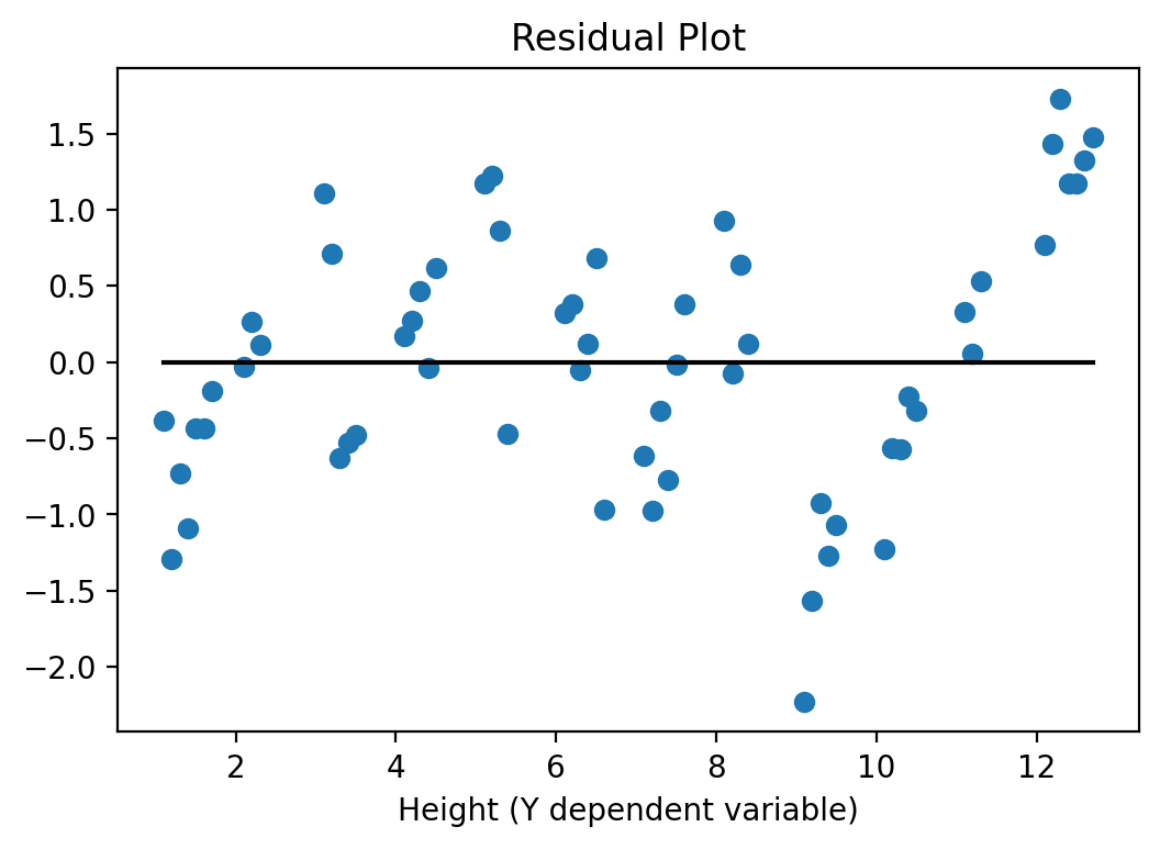
And here is the residual plot again to check for heteroskedasticity:
yv = y['Height'].values
y_hatv = res.predict(X).values  # Predicts y-hat based on all X values in data
residualsv = yv - y_hatv

fig, ax = plt.subplots()
ax.set_title('Residual Plot')
ax.plot(yv, residualsv, 'o', label = 'data')
ax.plot(yv, np.zeros(len(yv)),'k-')
ax.set_xlabel('Height (Y dependent variable)')
plt.show()
11.5. Measures of Non-Linear Relationship
We next demonstrate how to run Probit and Logit regressions. These
type of regression models are used when the dependent variable is a categorical
0/1 variable. If you instead ran a simple linear OLS regression on such a
variable, the possible predictions from this linear probability model could
fall outside of the [0,1] range. The Probit and Logit specifications
ensure that predictions are probabilities that will fall within the [0,1]
range.
Make sure that you have already downloaded the Excel data file
Lecture_Data_Excel_c.xlsx.
We next import the Excel file data directly from Excel using the
pd.read_excel() function from Pandas.
Important
In order for this to work you need to make sure that the xlrd package is
installed. Open a terminal window and type:
conda install xlrd
Press yes at the prompt and it will install the package.
You can now use the command. It is important to specify the Excel Sheet that you want to import data from since an Excel file can have multiple spreadsheets inside.
In our example the data resides in the sheet with the name binary. So we
specify this in the excel_read() function.
# Read entire excel spreadsheet
filepath = 'Lecture_Data/'
df = pd.read_excel(filepath + "Lecture_Data_Excel_c.xlsx", 'binary')

# Check how many sheets we have inside the excel file
#xl.sheet_names

# Pick one sheet and define it as your DataFrame by parsing a sheet
#df = xl.parse("binary")

print(df.head())

# rename the 'rank' column because there is also a DataFrame method called 'rank'
df.columns = ["admit", "gre", "gpa", "prestige"]
   admit  gre   gpa  rank
0      0  380  3.61     3
1      1  660  3.67     3
2      1  800  4.00     1
3      1  640  3.19     4
4      0  520  2.93     4
We next make dummies out of the rank variable.
# dummify rank
dummy_ranks = pd.get_dummies(df['prestige'], prefix='d_prest')

# Join dataframes
df = df.join(dummy_ranks)
print(df.head())
   admit  gre   gpa  prestige  d_prest_1  d_prest_2  d_prest_3
d_prest_4
0      0  380  3.61         3          0          0          1
0
1      1  660  3.67         3          0          0          1
0
2      1  800  4.00         1          1          0          0
0
3      1  640  3.19         4          0          0          0
1
4      0  520  2.93         4          0          0          0
1
11.5.1. Logit
We now estimate a Logit model as follows:
# Import the correct version of statsmodels
import statsmodels.api as sm
from patsy import dmatrices

y, X = dmatrices('admit ~ gre + gpa + d_prest_2 + d_prest_3 + d_prest_4', data=df, return_type='dataframe')

# Define the model
logit = sm.Logit(y, X)

# fit the model
res = logit.fit()

# Print results
print(res.summary())
Optimization terminated successfully.
         Current function value: 0.573147
         Iterations 6
                           Logit Regression Results
==============================================================================
Dep. Variable:                  admit   No. Observations:
400
Model:                          Logit   Df Residuals:
394
Method:                           MLE   Df Model:
5
Date:                Thu, 12 May 2022   Pseudo R-squ.:
0.08292
Time:                        15:51:24   Log-Likelihood:
-229.26
converged:                       True   LL-Null:
-249.99
Covariance Type:            nonrobust   LLR p-value:
7.578e-08
==============================================================================
                 coef    std err          z      P>|z|      [0.025
0.975]
------------------------------------------------------------------------------
Intercept     -3.9900      1.140     -3.500      0.000      -6.224
-1.756
gre            0.0023      0.001      2.070      0.038       0.000
0.004
gpa            0.8040      0.332      2.423      0.015       0.154
1.454
d_prest_2     -0.6754      0.316     -2.134      0.033      -1.296
-0.055
d_prest_3     -1.3402      0.345     -3.881      0.000      -2.017
-0.663
d_prest_4     -1.5515      0.418     -3.713      0.000      -2.370
-0.733
==============================================================================
A Slightly different summary
print(res.summary2())
                         Results: Logit
=================================================================
Model:              Logit            Pseudo R-squared: 0.083
Dependent Variable: admit            AIC:              470.5175
Date:               2022-05-12 15:51 BIC:              494.4663
No. Observations:   400              Log-Likelihood:   -229.26
Df Model:           5                LL-Null:          -249.99
Df Residuals:       394              LLR p-value:      7.5782e-08
Converged:          1.0000           Scale:            1.0000
No. Iterations:     6.0000
------------------------------------------------------------------
               Coef.   Std.Err.     z     P>|z|    [0.025   0.975]
------------------------------------------------------------------
Intercept     -3.9900    1.1400  -3.5001  0.0005  -6.2242  -1.7557
gre            0.0023    0.0011   2.0699  0.0385   0.0001   0.0044
gpa            0.8040    0.3318   2.4231  0.0154   0.1537   1.4544
d_prest_2     -0.6754    0.3165  -2.1342  0.0328  -1.2958  -0.0551
d_prest_3     -1.3402    0.3453  -3.8812  0.0001  -2.0170  -0.6634
d_prest_4     -1.5515    0.4178  -3.7131  0.0002  -2.3704  -0.7325
=================================================================
And here is the residual plot again to check for heteroskedasticity:
yv = y['admit'].values
y_hatv = res.predict(X).values  # Predicts y-hat based on all X values in data
residualsv = yv - y_hatv

fig, ax = plt.subplots()
ax.set_title('Residual Plot')
ax.plot(yv, residualsv, 'o', label = 'data')
ax.plot(yv, np.zeros(len(yv)),'k-')
ax.set_xlabel('admit (Y dependent variable)')
plt.show()
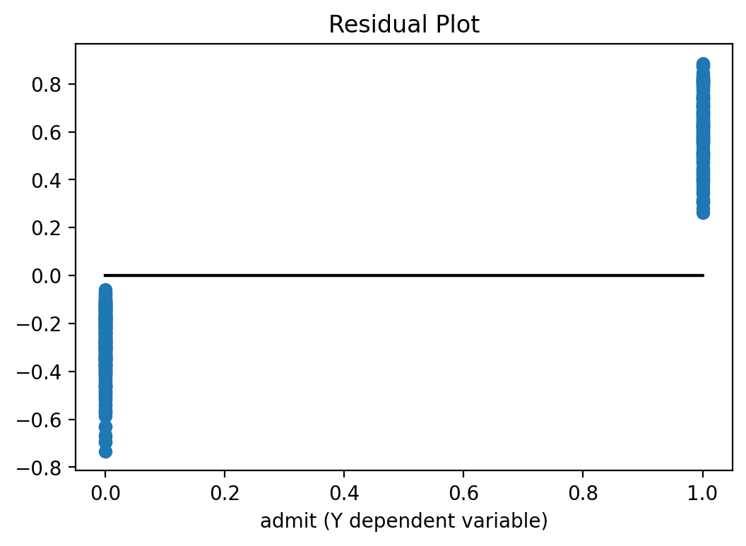
Not surprisingly we see that since the dependent variable can only take on the values 0 or 1, the residual plot shows only residuals at these two locations.
11.5.2. Probit
If you want to run a Probit regression, you can do:
import statsmodels.api as sm
from patsy import dmatrices

y, X = dmatrices('admit ~ gre + gpa + d_prest_2 + d_prest_3 + d_prest_4', data=df, return_type='dataframe')
# Define the model
probit = sm.Probit(y, X)

# Fit the model
res = probit.fit()

# Print results
print(res.summary())
Optimization terminated successfully.
         Current function value: 0.573016
         Iterations 5
                          Probit Regression Results
==============================================================================
Dep. Variable:                  admit   No. Observations:
400
Model:                         Probit   Df Residuals:
394
Method:                           MLE   Df Model:
5
Date:                Thu, 12 May 2022   Pseudo R-squ.:
0.08313
Time:                        15:51:25   Log-Likelihood:
-229.21
converged:                       True   LL-Null:
-249.99
Covariance Type:            nonrobust   LLR p-value:
7.219e-08
==============================================================================
                 coef    std err          z      P>|z|      [0.025
0.975]
------------------------------------------------------------------------------
Intercept     -2.3868      0.674     -3.541      0.000      -3.708
-1.066
gre            0.0014      0.001      2.120      0.034       0.000
0.003
gpa            0.4777      0.195      2.444      0.015       0.095
0.861
d_prest_2     -0.4154      0.195     -2.126      0.033      -0.798
-0.032
d_prest_3     -0.8121      0.209     -3.893      0.000      -1.221
-0.403
d_prest_4     -0.9359      0.246     -3.810      0.000      -1.417
-0.454
==============================================================================
A Slightly different summary
print(res.summary2())
                         Results: Probit
=================================================================
Model:              Probit           Pseudo R-squared: 0.083
Dependent Variable: admit            AIC:              470.4132
Date:               2022-05-12 15:51 BIC:              494.3620
No. Observations:   400              Log-Likelihood:   -229.21
Df Model:           5                LL-Null:          -249.99
Df Residuals:       394              LLR p-value:      7.2189e-08
Converged:          1.0000           Scale:            1.0000
No. Iterations:     5.0000
------------------------------------------------------------------
               Coef.   Std.Err.     z     P>|z|    [0.025   0.975]
------------------------------------------------------------------
Intercept     -2.3868    0.6741  -3.5408  0.0004  -3.7080  -1.0656
gre            0.0014    0.0006   2.1200  0.0340   0.0001   0.0026
gpa            0.4777    0.1955   2.4441  0.0145   0.0946   0.8608
d_prest_2     -0.4154    0.1954  -2.1261  0.0335  -0.7983  -0.0325
d_prest_3     -0.8121    0.2086  -3.8934  0.0001  -1.2210  -0.4033
d_prest_4     -0.9359    0.2456  -3.8101  0.0001  -1.4173  -0.4545
=================================================================
11.6. Tutorials
Some of the notes above are summaries of these tutorials: