10. Working with Data I: Data Cleaning
We use the Pandas package for data work. We can import the Pandas
library using the import statement. Pandas allows easy organization of
data in the spirit of DataFrame concept in R. You can think of a
DataFrame as an array with labels similar to an Excel spreadsheet.
A DataFrame can be created in the following ways:
From another DataFrame
From a
numpyarrayFrom lists
From another
pandasdata structure calledserieswhich is basically a one dimensional DataFrame, i.e., a column or row of a matrixFrom a file like a CSV file etc.
Later in this chapter we will be working with two data sets. You can download them from here:
Or the Excel version of it:
Here is a second data set in comma separated (.csv) format:
10.1. Create Dataframe from Multiple Lists
If you scrape information from a website or a pdf document, you often end up
with your data stored across various lists. Sometimes these lists are simply
holding the column information of a specific variable, sometimes the lists are
nested lists, where one list contains the information of all variables per
observation. pandas is intelligent enough (usually) to handle them all in a
very similar way. I next illustrate the two most often found list structures in
data work.
10.1.1. Every List Holds Information of a Separate Variable
Let us assume you observe information about 4! people. The unit of observation is therefore a person. For each person you know the name, age, and the city where they live. This information is stored in 3! separate lists.
There is an easy way to combine these lists into a Dataframe for easy statistical analysis. The process has two steps:
Use the
zip()command to combine the listsAssign the “zipped” lists to a Pandas Dataframe
import pandas as pd

names = ['Katie', 'Nick', 'James', 'Eva']
ages = [32, 32, 36, 31]
locations = ['London', 'Baltimore', 'Atlanta', 'Madrid']

# Now zip the lists together
zipped = list(zip(names, ages, locations))

# Assign the zipped lists into a Dataframe
myData = pd.DataFrame(zipped, columns=['Name', 'Age', 'Location'])
print(myData)
    Name  Age   Location
0  Katie   32     London
1   Nick   32  Baltimore
2  James   36    Atlanta
3    Eva   31     Madrid
10.1.2. Every List Holds Information of one Unit of Observation
In this example, the information is stored per person. So each person is stored in a list that contains all 3! variables. Then these person lists are stored in another list. We now are dealing with a nested list.
The steps to move the information from the lists into a Dataframe are pretty much the same. Pandas is intelligent in that way and recognizes the structure of the data.
Again the process has two steps:
Use the
zip()command to combine the listsAssign the “zipped” lists to a Pandas Dataframe
import pandas as pd

# This is the structure of your data
data = [['Katie', 32, 'London'], ['Nik', 32, 'Toronto'], ['James', 36, 'Atlanta'], ['Evan', 31, 'Madrid']]

# Assign the multi-dimensional (or nested) list to Dataframe
myData = pd.DataFrame(data, columns=['Name', 'Age', 'Location'])
print(myData)
    Name  Age Location
0  Katie   32   London
1    Nik   32  Toronto
2  James   36  Atlanta
3   Evan   31   Madrid
10.2. Read Small Data Set from a Comma Separated (.csv) File
It is more common that your data is stored in a file such as a text file, Excel spreadsheet, or a file format of some other data management software such as Stata, R, SAS, or SPSS. The Pandas library does provide you with routines (i.e., commands) that will allow you to import data directly from the most common file formats.
In our first example, we will work with data stored as a comma separated file, called
Lecture_Data_Excel_a.csv.
We first import this file using the pd.read_csv command from the Pandas library.
import numpy as np
import matplotlib.pyplot as plt
import pandas as pd
from scipy import stats as st
import math as m
import seaborn as sns
import time  # Imports system time module to time your script

plt.close('all')  # close all open figures
# Read in small data from .csv file
# Filepath
filepath = 'Lecture_Data/'
# In windows you can also specify the absolute path to your data file
# filepath = 'C:/Dropbox/Towson/Teaching/3_ComputationalEconomics/Lectures/Lecture_Data/'

# ------------- Load data --------------------
df = pd.read_csv(filepath + 'Lecture_Data_Excel_a.csv', dtype={'Frequency': float})

# Let's have a look at it.
print(df)
                 Area  Frequency  Unnamed: 2  Unnamed: 3
0          Accounting       73.0         NaN         NaN
1             Finance       52.0         NaN         NaN
2  General management       36.0         NaN         NaN
3     Marketing sales       64.0         NaN         NaN
4               other       28.0         NaN         NaN
Alternatively we could have use the following command:
df = pd.read_table(filepath + 'Lecture_Data_Excel_a.csv', sep=',')

# Let's have a look at it.
print(df)
                 Area  Frequency  Unnamed: 2  Unnamed: 3
0          Accounting         73         NaN         NaN
1             Finance         52         NaN         NaN
2  General management         36         NaN         NaN
3     Marketing sales         64         NaN         NaN
4               other         28         NaN         NaN
The best way to import Excel files directly is probably to use the built in
importer in Pandas.
Important
In order for this to work you need to make sure that the xlrd package is
installed. Open a terminal window and type:
conda install xlrd
Press yes at the prompt and it will install the package.
You can use it as follows:
# Read entire excel spreadsheet
df = pd.read_excel(filepath + 'Lecture_Data_Excel_a.xlsx', \
     sheet_name = 'Lecture_Data_Excel_a', header = 0, usecols = 'A:D')

# Let's have a look at it.
print(df)
                 Area  Frequency  Unnamed: 2  Unnamed: 3
0          Accounting         73         NaN         NaN
1             Finance         52         NaN         NaN
2  General management         36         NaN         NaN
3     Marketing sales         64         NaN         NaN
4               other         28         NaN         NaN
Note how I also specified the excel sheet_name this is convenient in case you have more complex Excel spreadsheets with multiple tabs in it.
The DataFrame has an index for each row and a column header. We can query a DataFrame as follows:
print('Shape', df.shape)
print('-------------------------')
print('Number of rows', len(df))
print('-------------------------')
print('Column headers', df.columns)
print('-------------------------')
print('Data types', df.dtypes)
print('-------------------------')
print('Index', df.index)
print('-------------------------')
Shape (5, 4)
-------------------------
Number of rows 5
-------------------------
Column headers Index(['Area', 'Frequency', 'Unnamed: 2', 'Unnamed:
3'], dtype='object')
-------------------------
Data types Area           object
Frequency       int64
Unnamed: 2    float64
Unnamed: 3    float64
dtype: object
-------------------------
Index RangeIndex(start=0, stop=5, step=1)
-------------------------
Drop column 3 and 4 and let’s have a look at the data again.
# axis = 1 means that you are dropping a column
df.drop('Unnamed: 2', axis=1, inplace=True)

df.drop('Unnamed: 3', axis=1, inplace=True)

# Let's have a look at it, it's a nested list
print(df)
                 Area  Frequency
0          Accounting         73
1             Finance         52
2  General management         36
3     Marketing sales         64
4               other         28
Warning
Sometimes column headers have white spaces in them. It is probably a good idea
to remove all white spaces from header names. You can use the replace()
command to accomplish this:
df.columns = df.columns.str.replace('\s+', '', regex=True)
The \s+ is a regular expression which is basically a pattern matching
language. The s stands for space and the + means look for one or more
spaces and replace them with '', well, nothing i.e. a blank string.
We can make new columns using information from the existing columns.
Note
Making new columns in the DataFrame is very similar to making new
variables in Stata using the generate or gen command.
More specifically, we next generate a new variable called relFrequency that contains the relative
frequencies.
# Make new column with relative frequency
df['relFrequency'] = df['Frequency']/df['Frequency'].sum()

# Let's have a look at it, it's a nested list
print(df)
                 Area  Frequency  relFrequency
0          Accounting         73      0.288538
1             Finance         52      0.205534
2  General management         36      0.142292
3     Marketing sales         64      0.252964
4               other         28      0.110672
We can also just grab the relative frequencies out of the DataFrame and store it
in the familiar a numpy array. This is now a vector. You can only do this if
the information in the column is only numbers.
xv = df['relFrequency'].values

print('Array xv is:', xv)
Array xv is: [0.28853755 0.2055336 0.14229249 0.25296443 0.11067194]
You can now do simple calculations with this vector as you did in the previous chapters such as:
print('The sum of the vector xv is: ', xv.sum())
The sum of the vector xv is: 1.0
Let us make an additional column so we have more data to play with:
df['random'] = df['Frequency']/np.sqrt(df['Frequency'].sum())

# Let's have a look at it.
print(df)
                 Area  Frequency  relFrequency    random
0          Accounting         73      0.288538  4.589471
1             Finance         52      0.205534  3.269212
2  General management         36      0.142292  2.263301
3     Marketing sales         64      0.252964  4.023646
4               other         28      0.110672  1.760345
10.3. Some Pandas Tricks
10.3.1. Renaming Variables
For renaming column names we use a dictionary.
Note
Remember, dictionaries are similar to lists but the indexing of the elements of a dictionary is not done with 0,1,2, etc. but we user defined keys so that a dictionary consists of key - value pairs such as:
{'key1': value1, 'key2': value2, ... }
It works as follows. You see how the dictionary that you hand-in here defines
the old column name as key and the new column name as the associated
value.
df = df.rename(columns={'Area': 'area', 'Frequency': 'absFrequency'})

print(df.head(3))
                 area  absFrequency  relFrequency    random
0          Accounting            73      0.288538  4.589471
1             Finance            52      0.205534  3.269212
2  General management            36      0.142292  2.263301
The head(x) method allows us to print x rows from the top of the
DataFrame, whereas the tail(x) method does the same from the bottom of
the DataFrame.
10.3.2. Dropping and Adding Columns
# Drop a column first so everything fits
df = df.drop('random', axis=1)

# Create a new column with some missing values
df['team'] = pd.Series([2,4, np.NaN,6,10], index=df.index)

# or insert new column at specific location
df.insert(loc=2, column='position', value=[np.NaN,1, np.NaN,1,3])

print(df)
                 area  absFrequency  position  relFrequency  team
0          Accounting            73       NaN      0.288538   2.0
1             Finance            52       1.0      0.205534   4.0
2  General management            36       NaN      0.142292   NaN
3     Marketing sales            64       1.0      0.252964   6.0
4               other            28       3.0      0.110672  10.0
10.3.3. Missing Values of NaN’s
Count NaNs
Count the number of rows with missing values.
nans = df.shape[0] - df.dropna().shape[0]
print('{} rows have missing values'.format(nans))
2 rows have missing values
Select rows with NaNs or overwrite NaNs
If you want to select the rows with missing values you can index them with the
isnull() method.
print(df[df.isnull().any(axis=1)])
                 area  absFrequency  position  relFrequency  team
0          Accounting            73       NaN      0.288538   2.0
2  General management            36       NaN      0.142292   NaN
Or if you want to search specific columns for missing values you can do
print(df[df['team'].isnull()])
                 area  absFrequency  position  relFrequency  team
2  General management            36       NaN      0.142292   NaN
Or if you want to grab all the rows without missing observations you can index
the dataframe with the notnull() method.
print(df[df['team'].notnull()])
              area  absFrequency  position  relFrequency  team
0       Accounting            73       NaN      0.288538   2.0
1          Finance            52       1.0      0.205534   4.0
3  Marketing sales            64       1.0      0.252964   6.0
4            other            28       3.0      0.110672  10.0
Delete rows with NaNs
print(df.dropna())
              area  absFrequency  position  relFrequency  team
1          Finance            52       1.0      0.205534   4.0
3  Marketing sales            64       1.0      0.252964   6.0
4            other            28       3.0      0.110672  10.0
You can also reassign it to the orignal DataFrame or assign a new one.
df2 = df.dropna()
print(df2)
              area  absFrequency  position  relFrequency  team
1          Finance            52       1.0      0.205534   4.0
3  Marketing sales            64       1.0      0.252964   6.0
4            other            28       3.0      0.110672  10.0
Overwriting NaN with specific values
If we want to overwrite the NaN entries with values we can use the
fillna() method. In this example we replace all missing values with zeros.
df.fillna(value=0, inplace=True)
print(df)
                 area  absFrequency  position  relFrequency  team
0          Accounting            73       0.0      0.288538   2.0
1             Finance            52       1.0      0.205534   4.0
2  General management            36       0.0      0.142292   0.0
3     Marketing sales            64       1.0      0.252964   6.0
4               other            28       3.0      0.110672  10.0
10.3.4. Dropping and Adding Rows to a DataFrame
We can use the append() method to add rows to the DataFrame.
df = df.append(pd.Series(
                [np.nan]*len(df.columns), # Fill cells with NaNs
                index=df.columns),
                ignore_index=True)

print(df.tail(3))
              area  absFrequency  position  relFrequency  team
3  Marketing sales          64.0       1.0      0.252964   6.0
4            other          28.0       3.0      0.110672  10.0
5              NaN           NaN       NaN           NaN   NaN
We can then fill this empty row with data.
df.loc[df.index[-1], 'area'] = 'Economics'
df.loc[df.index[-1], 'absFrequency'] = 25
print(df)
                 area  absFrequency  position  relFrequency  team
0          Accounting          73.0       0.0      0.288538   2.0
1             Finance          52.0       1.0      0.205534   4.0
2  General management          36.0       0.0      0.142292   0.0
3     Marketing sales          64.0       1.0      0.252964   6.0
4               other          28.0       3.0      0.110672  10.0
5           Economics          25.0       NaN           NaN   NaN
If you want to drop this row you can:
print(df.drop(5), 0)
                 area  absFrequency  position  relFrequency  team
0          Accounting          73.0       0.0      0.288538   2.0
1             Finance          52.0       1.0      0.205534   4.0
2  General management          36.0       0.0      0.142292   0.0
3     Marketing sales          64.0       1.0      0.252964   6.0
4               other          28.0       3.0      0.110672  10.0 0
If you want the change to be permanent you need to either use the
df.dropb(5, inplace=True) option or you reassign the DataFrame to itself
df = df.drop(5). The default dimension for dropping data is the row in the
DataFrame, so you do not need to specify the , 0 part in the drop command.
However, if you drop a column, then you need the dimension specifier , 1.
10.3.5. Dropping Rows Based on Conditions
Before running a regression, a researcher might like to drop certain observations that are clearly not correct such as negative age observations for instance.
Let us assume that in our current dataframe we have information that tells us
that a position variable must be strictly positive and cannot be zero. This
would mean that row 0 and row 2 would need to be dropped from our dataframe.
Before we mess up our dataframe, let’s make a new one and then drop row 0 and 2
based on the value condition of variable position.
df_temp = df

print(df_temp)
                 area  absFrequency  position  relFrequency  team
0          Accounting          73.0       0.0      0.288538   2.0
1             Finance          52.0       1.0      0.205534   4.0
2  General management          36.0       0.0      0.142292   0.0
3     Marketing sales          64.0       1.0      0.252964   6.0
4               other          28.0       3.0      0.110672  10.0
5           Economics          25.0       NaN           NaN   NaN
Now drop the rows with a position variable value of zero or less.
df_temp = df_temp[df_temp['position']>0]
print(df_temp)
              area  absFrequency  position  relFrequency  team
1          Finance          52.0       1.0      0.205534   4.0
3  Marketing sales          64.0       1.0      0.252964   6.0
4            other          28.0       3.0      0.110672  10.0
As you can see we accomplished this by “keeping” the observations for which the
position value is strictly positive as opposed to “dropping” the negative
ones.
And also let’s make sure that the original dataframe is still what it was.
print(df)
                 area  absFrequency  position  relFrequency  team
0          Accounting          73.0       0.0      0.288538   2.0
1             Finance          52.0       1.0      0.205534   4.0
2  General management          36.0       0.0      0.142292   0.0
3     Marketing sales          64.0       1.0      0.252964   6.0
4               other          28.0       3.0      0.110672  10.0
5           Economics          25.0       NaN           NaN   NaN
10.3.6. Sorting and Reindexing DataFrames
We next sort the DataFrame by a certain column (from highest to lowest) using
the sort_values() DataFrame method.
Warning
The old pandas method/function .sort() was replaced with
.sort_values() and does not work anymore in newer versions of pandas.
df.sort_values('absFrequency', ascending=False, inplace=True)
print(df)
                 area  absFrequency  position  relFrequency  team
0          Accounting          73.0       0.0      0.288538   2.0
3     Marketing sales          64.0       1.0      0.252964   6.0
1             Finance          52.0       1.0      0.205534   4.0
2  General management          36.0       0.0      0.142292   0.0
4               other          28.0       3.0      0.110672  10.0
5           Economics          25.0       NaN           NaN   NaN
The inplace=True option will immediately overwrite the DataFrame df
with the new, sorted, one. If you set inplace=False you would have to
assign a new DataFrame in order to see the changes:
df1 = df.sort_values('absFrequency', ascending=False, inplace=False)
Where df1 would now be the sorted DataFrame and the original df
DataFrame would still be unsorted.
Note
However, we now have two objects with
identical data in it. This is often redundant and can eventually become a memory problem if the DataFrames are
very large. Setting inplace=True is probably a good default setting.
If we want we could then reindex the DataFrame according to the new sort order.
df.index = range(len(df.index))
print(df)
                 area  absFrequency  position  relFrequency  team
0          Accounting          73.0       0.0      0.288538   2.0
1     Marketing sales          64.0       1.0      0.252964   6.0
2             Finance          52.0       1.0      0.205534   4.0
3  General management          36.0       0.0      0.142292   0.0
4               other          28.0       3.0      0.110672  10.0
5           Economics          25.0       NaN           NaN   NaN
10.3.7. Merging DataFrames or Adding Columns
Let us create a new DataFrame that has the variable team in common with the previous
DataFrame. This new DataFrame contains additional team information that we
would like to merge into the original DataFrame.
First redefine the orginal DataFrame:
df= pd.DataFrame({'area': ['Accounting','Marketing','Finance','Management', 'other'],\
                  'absFrequency': [73,64,52,36,28], \
                  'position': [0,1,1,0,3], \
                  'relFrequency': [0.28,0.25,0.20,0.14,0.11], \
                  'team': [2,6,4,0,10]})

print(df)
         area  absFrequency  position  relFrequency  team
0  Accounting            73         0          0.28     2
1   Marketing            64         1          0.25     6
2     Finance            52         1          0.20     4
3  Management            36         0          0.14     0
4       other            28         3          0.11    10
Second, we define the new DataFrame and add some values to it:
df_team = pd.DataFrame({'team': [3,4,5,6,7,8,9,10], \
                        'sales': [500,300,250,450,345,123,432,890]})

print(df_team)
   team  sales
0     3    500
1     4    300
2     5    250
3     6    450
4     7    345
5     8    123
6     9    432
7    10    890
This new DataFrame contains some sales information for each team.
Before we merge in the new info we drop the area column so that
the DataFrame fits on the screen. We now work with the following two
dataframes.
df = df.drop('area', axis=1)
print('-----------------------------')
print('First, main,  DataFrame: LEFT')
print('-----------------------------')
print(df)
print('')
print('-----------------------------')
print('Second new DataFrame: RIGHT')
print('-----------------------------')
print(df_team)
-----------------------------
First, main,  DataFrame: LEFT
-----------------------------
   absFrequency  position  relFrequency  team
0            73         0          0.28     2
1            64         1          0.25     6
2            52         1          0.20     4
3            36         0          0.14     0
4            28         3          0.11    10

-----------------------------
Second new DataFrame: RIGHT
-----------------------------
   team  sales
0     3    500
1     4    300
2     5    250
3     6    450
4     7    345
5     8    123
6     9    432
7    10    890
When merging two dataframes we need to find a common variable that appears in
both DataFrames along which we can connect them. In our example we use the
team column as merge-key or key-variable because it appears in both
DataFrames. We have now four different options for merging the two DataFrames.
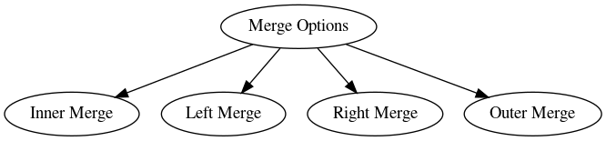
Note
Merge Summary
The inner merge only keeps observations that are present in both DataFrames.
The left merge keeps all of the observations of the original (or main DataFrame) and adds the new information on the left if available.
The right merge only keeps info from the new DataFrame and adds the info of the original main DataFrame.
The outer merge method merges by team whenever possible but keeps the info from both DataFrames, even for observations where no merge/overlap occurred.
Now we do it step my step. Inner merge first. As you will see now, the inner merge only keeps observations that are present in both DataFrames. This is often too restrictive as many observations will be dropped.
print('Inner Merge')
print('-----------')
print(pd.merge(df, df_team, on='team', how='inner'))
Inner Merge
-----------
   absFrequency  position  relFrequency  team  sales
0            64         1          0.25     6    450
1            52         1          0.20     4    300
2            28         3          0.11    10    890
The left merge keeps the original (or main DataFrame) and adds the new information on the left. When it cannot find a team number in the main DataFrame it simply drops the info from the new DataFrame.
print('Left Merge')
print('----------')
print(pd.merge(df, df_team, on='team', how='left'))
Left Merge
----------
   absFrequency  position  relFrequency  team  sales
0            73         0          0.28     2    NaN
1            64         1          0.25     6  450.0
2            52         1          0.20     4  300.0
3            36         0          0.14     0    NaN
4            28         3          0.11    10  890.0
The right merge only keeps info from the new DataFrame and adds the info of the original main DataFrame.
print('Right Merge')
print('-----------')
print(pd.merge(df, df_team, on='team', how='right'))
Right Merge
-----------
   absFrequency  position  relFrequency  team  sales
0           NaN       NaN           NaN     3    500
1          52.0       1.0          0.20     4    300
2           NaN       NaN           NaN     5    250
3          64.0       1.0          0.25     6    450
4           NaN       NaN           NaN     7    345
5           NaN       NaN           NaN     8    123
6           NaN       NaN           NaN     9    432
7          28.0       3.0          0.11    10    890
The outer merge method merges by team whenever possible but keeps the info from both DataFrames, even for observations where no merge/overlap occurred.
print('Outer Merge')
print('-----------')
print(pd.merge(df, df_team, on='team', how='outer'))
Outer Merge
-----------
   absFrequency  position  relFrequency  team  sales
0          73.0       0.0          0.28     2    NaN
1          64.0       1.0          0.25     6  450.0
2          52.0       1.0          0.20     4  300.0
3          36.0       0.0          0.14     0    NaN
4          28.0       3.0          0.11    10  890.0
5           NaN       NaN           NaN     3  500.0
6           NaN       NaN           NaN     5  250.0
7           NaN       NaN           NaN     7  345.0
8           NaN       NaN           NaN     8  123.0
9           NaN       NaN           NaN     9  432.0
10.3.8. Converting Column Types
When converting text into a DataFrame to conduct statistical analysis it is sometimes necessary to convert a numbers column that is still a string, into floats, so that we can do math. Let’s drop some more columns first so the DataFrame fits nicely in the output window.
df = df.drop('absFrequency', axis=1)
# Let's have a look at it, it's a nested list
print(df)
   position  relFrequency  team
0         0          0.28     2
1         1          0.25     6
2         1          0.20     4
3         0          0.14     0
4         3          0.11    10
We now generate a column of “words” or “strings” that happen do be numbers. Since they are defined as words, we cannot run statistical analysis on these numbers yet.
df['string'] = pd.Series(['2','40','34','6','10'], index=df.index)

# Print DataFrame
print(df)

# Print summary statistics
print(df.describe())
   position  relFrequency  team string
0         0          0.28     2      2
1         1          0.25     6     40
2         1          0.20     4     34
3         0          0.14     0      6
4         3          0.11    10     10
       position  relFrequency       team
count  5.000000      5.000000   5.000000
mean   1.000000      0.196000   4.400000
std    1.224745      0.071624   3.847077
min    0.000000      0.110000   0.000000
25%    0.000000      0.140000   2.000000
50%    1.000000      0.200000   4.000000
75%    1.000000      0.250000   6.000000
max    3.000000      0.280000  10.000000
We first need to reassign the data type of the string column. We then
rename the column and print summary statistics.
# Transform strings into floats, i.e., words into numbers
df['string'] = df['string'].astype(float)

# Rename the column
df = df.rename(columns={'string': 'salary'})

# Print summary statistics
print(df.describe())
       position  relFrequency       team     salary
count  5.000000      5.000000   5.000000   5.000000
mean   1.000000      0.196000   4.400000  18.400000
std    1.224745      0.071624   3.847077  17.343587
min    0.000000      0.110000   0.000000   2.000000
25%    0.000000      0.140000   2.000000   6.000000
50%    1.000000      0.200000   4.000000  10.000000
75%    1.000000      0.250000   6.000000  34.000000
max    3.000000      0.280000  10.000000  40.000000
10.3.9. Replacing Values in a DataFrame Conditional on Criteria
If we need to replace values in a DataFrame based on certain criteria it is often more efficient to use indexing as opposed to loops. Let us first create a DataFrame with some random values:
df1 = pd.DataFrame(np.random.rand(10,5)*100)
print(df1)
           0          1          2          3          4
0  76.231650  73.856596  98.223677  37.419310  56.534611
1  93.020350  59.102390  87.029799   6.289979  81.704176
2  67.060606  30.773903  27.633734  35.819372  52.103559
3  80.603039  63.205036  16.050168  67.673033  19.890453
4  53.266469   8.721019  42.579826  36.000875  15.518005
5  20.139680  49.216850   9.924973  31.078271  77.523813
6  37.838850  65.905862  96.325081  99.530884  48.992624
7  52.408115  40.192827  60.132690  21.112231  52.065246
8  93.561547  36.599218  38.663248  56.510712  26.487473
9   8.446148  78.818387  74.815600  40.085175  90.895161
We next replace all the values in column 2 that are smaller than 30 with
the string low.
df1[1][(df1[1]<30)] = 'Low'
print(df1)
           0          1          2          3          4
0  76.231650  73.856596  98.223677  37.419310  56.534611
1  93.020350   59.10239  87.029799   6.289979  81.704176
2  67.060606  30.773903  27.633734  35.819372  52.103559
3  80.603039  63.205036  16.050168  67.673033  19.890453
4  53.266469        Low  42.579826  36.000875  15.518005
5  20.139680   49.21685   9.924973  31.078271  77.523813
6  37.838850  65.905862  96.325081  99.530884  48.992624
7  52.408115  40.192827  60.132690  21.112231  52.065246
8  93.561547  36.599218  38.663248  56.510712  26.487473
9   8.446148  78.818387  74.815600  40.085175  90.895161
We next replace all the values of column 4 that are larger than 70 with the
value 1000.
df1.loc[(df1[3]>70), 3] = 1000
print(df1)
           0          1          2            3          4
0  76.231650  73.856596  98.223677    37.419310  56.534611
1  93.020350   59.10239  87.029799     6.289979  81.704176
2  67.060606  30.773903  27.633734    35.819372  52.103559
3  80.603039  63.205036  16.050168    67.673033  19.890453
4  53.266469        Low  42.579826    36.000875  15.518005
5  20.139680   49.21685   9.924973    31.078271  77.523813
6  37.838850  65.905862  96.325081  1000.000000  48.992624
7  52.408115  40.192827  60.132690    21.112231  52.065246
8  93.561547  36.599218  38.663248    56.510712  26.487473
9   8.446148  78.818387  74.815600    40.085175  90.895161
And finally we can combine logical statements and replace values on a
combination of conditions. So let’s replace all the values in column 5 that
are between 20 and 80 with the string middle.
df1.loc[((df1[4]>20) & (df1[4]<80)), 4] = 'Middle'
print(df1)
           0          1          2            3          4
0  76.231650  73.856596  98.223677    37.419310     Middle
1  93.020350   59.10239  87.029799     6.289979  81.704176
2  67.060606  30.773903  27.633734    35.819372     Middle
3  80.603039  63.205036  16.050168    67.673033  19.890453
4  53.266469        Low  42.579826    36.000875  15.518005
5  20.139680   49.21685   9.924973    31.078271     Middle
6  37.838850  65.905862  96.325081  1000.000000     Middle
7  52.408115  40.192827  60.132690    21.112231     Middle
8  93.561547  36.599218  38.663248    56.510712     Middle
9   8.446148  78.818387  74.815600    40.085175  90.895161