9 Production Technology and Full Employment
This chapter covers a first discussion of the distinction of short-run and long-run time horizons. The short-run typically refers to the time period where prices are not able to adjust or adjust much. This is often referred to as price rigidity and plays a prominent part in modern macroeconomic models.
The long-run refers to a time period where prices can fully adjust to new market conditions. Prices are said to be flexible in the long-run. Price adjustments and prices being able to freely adjust are at the center of arguments for how free markets can reach efficient outcomes that are beneficial to households and other market participants.
9.1 Economic Schools of Thought
9.1.1 Classical Economist's Way of Thinking
Classical Economics is mostly concerned with long-run analysis. Remember, in the long-run prices can fully adjust to market conditions.
Classical economist believed that there are strong forces pushing the economy back to full employment after unemployment shocks occurred. As equilibrium is reached in the long-run, booms or busts are therefore only temporary.
- They are business cycle issues
- We can just "wait it out" as the markets adjust and move the economy back to full-employment. In a classical economist's view there is only a very limited role for government (i.e., ensuring property rights, national defense, providing some public goods).
Active fiscal policy---where the government tries to actively affect the business cycle (i.e., the ups and downs of GDP over time) through tax and spending policies---is often criticized by economists of the classical tradition as doing more harm than good.
In summary Classical Economics is long-run focused and
- Wages and prices adjust freely and quickly to all changes in demand and supply.
- Hence, we call this the long-run analysis.
- Markets adjust freely.
- Minor role for Government.
9.1.2 Keynesian Analysis: Short-Run
Keynes does not care about the long-run. His famous quote states: “In the long-run we are all dead.” The focus on the long-run that classical economists embrace, seems misguided if workers have trouble finding jobs right now.
Keynes therefore advocates an active fiscal policy and a focus on the short-run. In the short prices and wages seem to be “sticky”. Government intervention needed to adjust the econosmy back to equilibrium. According to Keynes we cannot afford to wait for the “long-run” where markets fix everything automatically through appropriate prices adjustments (as advocated by the classical school).
If the economy is in a slump, is there anything the government can do? Keynes' answer is yes. It typically involves fiscal policy, i.e., cutting taxes or increasing government spending or a combination of both. This type of policy is often referred to as deficit spending as cutting taxes and/or increasing the spending of government will invariably increase the deficit.
An important concept in discussing short-run and long-run effects is understanding the concept of Full Employment. An economy is at full employment when cyclical unemployement is zero (go back and read the chapter on the various types of unemployment again). This does not mean that everybody in the labor force is employed. We can still observe frictional and structural unemployment.
- Neoclassical anlaysis focuses on the long-run where all prices are fully flexible to adjust and where markets reach equilibrium allocations automatically through market forces and the resulting price adjustments.
- Keynesian analysis focuses on the short-run where prices are sticky. It advocates for an active role of government in an attempt to smooth out the business cycle and reduce unemployment.
- Full employment The economy is experiencing neither a boom nor a bust and there is zero cyclical unemployment.
- An economist advocates for a tax cut during a recession. Which economic school of thought does this economist follow?
9.2 Production Technology
How Much Does the Economy Produce? Production is typically measured using a production function. A production unit (or firm) produces goods and servies using input factors such as labor, capital, raw materials, land, etc.
The productivity of these inputs (or the effectiveness of the usage of input factors) depends on the level of technology in the economy which is referred to as total factor productivity or TFP.
9.2.1 The Representative Firm
In a macroeconomic model we often operate at the aggregate level. We assume that the economy is populated by countless smaller firms that are all identical in their basic makeup, i.e., they use capital and labor as input factors and produce an identical final good/service. This allows us to "add them all up" into a representative aggregate production unit or a representative firm.
This firm demands labor (\(N^d\)) and capital (\(K\)) in factor markets and pays a wage and an interest rate as compensation to the owners of labor and capital.
The choice of the firm about how much to produce is determined by its technology and a profit maximization motive. How much a firm is able to produce depends on the firm's total factor productivity \(A\) (think of this as the level of technology that is available to the firm) and the quantity of input factors such as capital \(K\) and labor \(N^d\). Formally, this can be written as the following production function:
\[Y=A \times F(K,N_{d}),\]
where A is the total factor productivity (TFP) which is a measure of overall effectiveness or technology!
Here is an example of a very specific production function:
\[Y= 10 \times K^\alpha \times N_{d}^{(1-\alpha)}.\]
The greek letter \(\alpha\) is the factor share of capital in production and \(1-\alpha\) is the factor share of labor in production. It is basically a factor that tells you how important capital is in relation to labor when producing output.
Let us assume that \(\alpha = 0.3\) and the firm uses 20 units of capital and 15 units of labor, then output would be:
\[Y= 10 \times 20^{0.3} \times 15^{(1-0.3)} = 163.5207536.\]
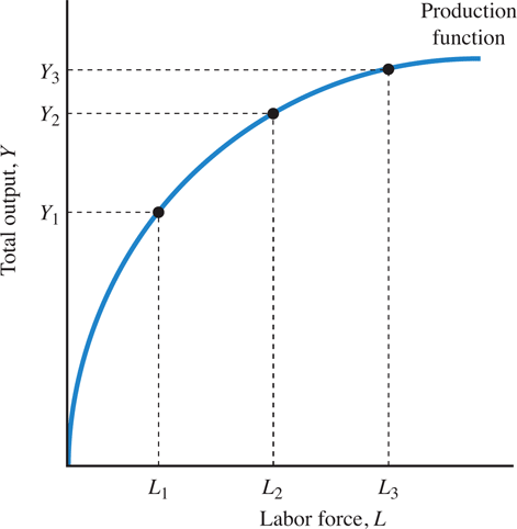
One of the properties of a typical production function in macroeconomics is diminishing returns to scale in factor inputs. This means that as a firm employs more and more of an input factor, while NOT increasing the other input factors, the output will increase BUT at a decreasing rate.
Figure 9.1 shows an example of diminishing (or decreasing) returns to scale in a production function where capital is fixed at a certain amount of capital \(\overline{K}\)
| Y (Output) | \(N_d\) (labor input) | Additional Output (MPN) |
|---|---|---|
| 1,000 | 1 | 1,000 |
| 1,500 | 2 | 500 |
| 1,900 | 3 | 400 |
| 2,200 | 4 | 300 |
From Table 9.1 you see that with this production function every additional labor unit produces less additional output than the previous labor unit. The first labor unit produces 1,000 units of output. The second labor unit that you add produces an additional 500 units for a total of 1,500 units. The third labor unit that you add produces an additional 400 units for a total of 1,900 units (with 3 workers employed). The fourth produces an additional 300 units. You see that the "additional units" you get keep decreasing, hence the name diminishing returns to scale if the capital input is held fixed!
The additional output is referred to as marginal product of labor or MPN. The additional output is decreasing as the firm hires more labor but keeps the amount of capital constant.
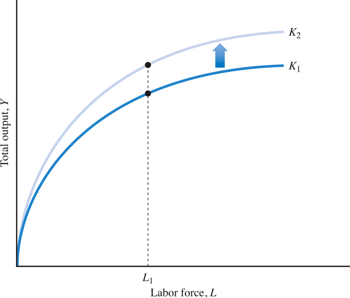
If, on the other hand, capital increases as well, then every unit of labor is producing more than before the capital increase. Figure 9.2 shows this case.
Returns to Scale Concepts
- As previously discussed, a standard production function in macroeconomics typically exhibits decreasing returns to scale (DRS) IF one of the input factors is held constant.
- A production function exihibits constant returns to scale (CRS) if, an increase in ALL of the input factors increases output at the same ratio.
So for example, if both labor and capital are doubled, then output will double as well. The concept of CRS embeds the notion of perfect reproduceability of a production unit, or perfect replication (or cloning) of a firm is assumed to be possible.
More formally a production function exhibits CRS if:
\[n \times Y=A\times F(n\times K,\mbox{ }n\times N^{d})\]
Here is an example
If n=2 then, if the production function is CRS, a doubling of ALL the input factors \((2\times K)\) and \((2\times N^{d})\) results in
\[2\times Y=A\times F(2\times K,\mbox{ }2\times N^{d})\]
a doubling of the output.
An often used function form in macroeconomics is the Cobb-Douglas production function:
\[Y=A\times K^{\alpha}\times N^{1-\alpha}\]
where the parameter \(\alpha\) measures the share of total income spent on capital and \((1-\alpha)\) measures the share of total income spent on labor input. Estimates from empirical studies have found that for the U.S. economy \(\alpha\) is around \(\frac{1}{3}\).
This is how the production function would then be written:
\[Y=A\times K^{0.3}\times N^{0.7}\]
Now, double all inputs, what happens to output?
\[Y_{new}=A\times\left(2\times K\right)^{0.3}\times\left(2\times N\right)^{0.7},\]\[\rightarrow Y_{new}=2^{0.3}\times2^{0.7}\times\left[A\times K^{0.3}\times N^{0.7}\right],\]\[\rightarrow Y_{new}=2^{\left(0.3+0.7\right)}\times Y=2\times Y.\]
As you can see, output has doubled as well.
The Properties of the production function \(Y=A\times F(K, N^{d})\) include:
- Output is increasing in its inputs, or: Y ↑ when either Nd ↑ or K ↑ or both
- The marginal product of labor decrease (MPL ↓) when labor input increases (Nd ↑) The MPL is the extra output that can be generated with an additional unit of labor. This return that additional workers generate decrease as more and more workers are added. Check again the discussion of diminishing returns to scale.
- The marginal product of capital decrease (MPK ↓) when the capital input increases (K ↑)
- The marginal product of labor increases (MPL ↑) when the input of captial increases (K ↑). In other words, more capital inputs, make workers more productive. The company's output per worker increases.
- A firm produces 4 units of output with 2 workers and 3 units of capital. This year the firm hires two more workers. Will output at the end of the year double?
9.3 Labor Markets
The amount of employment in an economy is determined by the demand and supply for labor. Firms demand labor, households supply labor. The amount of labor firms will hire depends on the real wage that firms have to pay for a labor unit (typically a work hour).
9.3.1 Wages and the Demand and Supply for Labor
The nominal wage rate paid to employees adjusted for changes in the price level. To understand the demand for labor, we use the marginal principle.
The marginal principle states that an economic activity is done up to the point where the marginal benefit of the activity is equal to the marginal cost that the activity cause. MB = MC.
The supply of labor is based on the decisions of workers. Changes in real wages have two different effects on the work-leisure trade-off:
- Substitution effect: a higher real wage causes workers to substitute work for leisure, so they work more hours.
- Income effect: a higher real wage rate increases real income, thus workers can afford to have more leisure time, so they work fewer hours.
Both effects work in opposite directions!
We typically assume (and it is empirically shown) that the substitution effect dominates the income effect which means that higher wages lead to more supply of labor. With this assumption in place, we can draw and upward sloping labor supply curve in a labor market graph. Figure 9.3 shows a labor demand and labor supply graph as well as a graph that depicts the labor market equilibrium at the equilibrium wage rate of $15.
9.3.2 Labor Market Equilibrium
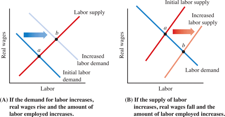
How would an increase in the stock of capital (i.e., machines, factories) affect the labor demand?
- Labor demand would shift to the right. Workers become more productive as more machines become available. Firms, with profit maximization in mind, would have an incentive to hire more workers for any given market wage rate than before the increase in capital.
- The increase in the demand for labor, a right shift, would increase the total hours worked and increase the real wage rate.
As long as full employment can be maintained, workers prefer a high capital stock as they then benefit from higher real wages.
This is not a story about machines replacing workers. This is a story of machines making workers more productive and hence workers will experience an increase in their real wage.
How would an increase in immigration affect the labor supply?
- It would lead to a right shift in the labor supply. For any given market wage, more labor hours would be supplied due to the increase in the number of potential workers.
- The new equilibrium would should an increase in the total hours worked and a decrease in the real wage rate.
Black Death in England
According to the research of Gregory Clark of the UC, Davis, the level of real wages for laborers in England was nearly the same in 1200 as it was in 1800. Yet, during the period from 1350 to 1550, they were higher—nearly 75 percent higher in 1450, for instance, than in 1200. Why were real wages temporarily so high during this period?
The simple answer was the bubonic plague—also known as the Black Death. Arrived from Asia in 1348 and caused a long decline in total population through the 1450s. With fewer workers, there was less labor supplied to the market. The result was higher real wages.
In the era before consistent and rapid technological advance, changes in population was the primary factor controlling living standards. As the economist Thomas Malthus (1766–1834) observed, social maladies such as the Black Death would temporarily raise living standards until higher living standards led to increased population.
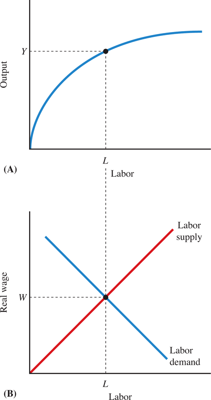
The demand and supply of labor determine the real wage, \(W^*\), and identify the level of employment, \(L^*\). That level of employment is used to determine the level of output \(Y^*\).
Full-employment output \(Y^*\) is the level of output that is produced when the labor market is in equilibrium. It is also known as potential output or long-run output.
At full-employment the cyclical unemployment rate is zero. There is still the frictional and structural unemployment rate present. The unemployment that is still present when the economy is at full-employment is referred to as the natural rate of unemployement. It is estimated that the natural rate of unemployment in the U.S. is around 4% - 5.5%.
So at full-employment in the U.S. we still observe an unemployment rate of about 4%!
9.3.3 Taxes on Labor
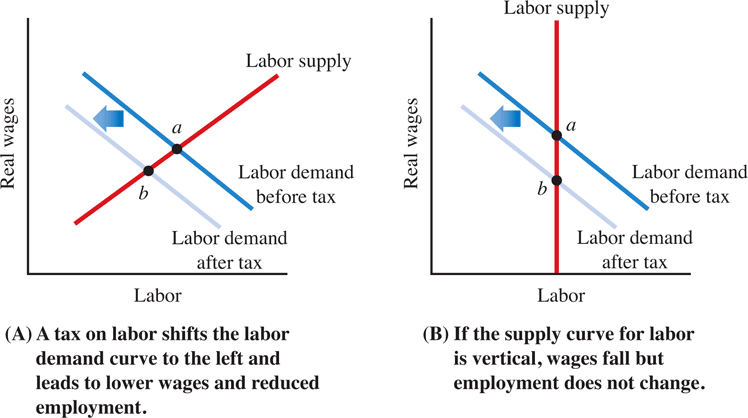
Labor supply in U.S. is close to vertical! This means that labor supply is very inelastic. Inelastic means, that labor supply does not respond strongly to changes in the wage rates in the aggregate. An increase in the wage rate will not entice people to work a whole lot more hours while a decrease in the wage rate will also not cause a large decrease in work hours supplied by households.
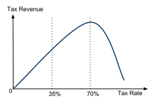
The Laffer Curve depicts the relationship between the income tax rate on the horizontal axes and government tax revenue on the vertical axis. The relationship is hump shaped. If taxes are very low and taxes increase then so does tax revenue.
However, there will be a point after which a further tax increase is so detrimental to workers incentive to work, that workers will drop out of the labor force and stop working due to high taxes. As a consequence the tax base will shrink, so that despite the higher tax rate, less tax can be collected by the government and tax revenue declines.
Estimating the peak of the Laffer curve is very difficult. It is different for every tax and depends on the structure of the economy as well as the institutions (economic and political) of a country. For instance, the labor supply response to an increase in the labor tax rate for instance would depend on the elasticity of labor supply to the net wage rate i.e. how responsive workers would be to changes in net wage on average. This average elasticity number depends on many factors such as: sector composition of an economy, perceptions of fairness of workers, worker representation, political climate, etc.
An estimate of the Laffer curve for the US from 2011 found that the optimal tax rate is around 73 percent. See: Diamond, Peter, and Emmanuel Saez. 2011. "The Case for a Progressive Tax: From Basic Research to Policy Recommendations." Journal of Economic Perspectives, 25 (4): 165-90. DOI: 10.1257/jep.25.4.165
An often heard argument is that lowering the tax rate would increase tax revenue. This is, at least in theory true, if an economy happens to be currently on the right side of the "hump" of the Laffer curve. If you are to the right of the hump, then a tax cut, can increase tax revenue.
However, this story usually requires that a tax cut will stimulate more work. Since we just learned earlier that in the U.S. the labor supply is very steep, a tax cut will not increase labor a whole lot.
Have a look at the secon panel of Figure 9.7. Changes in labor demand due to changes in the tax rate are not going to affect the equlibrium quantity of labor supplied. So the Laffer curve argument does not really work for income taxes in the U.S.
It might work for capital gains taxes though as capital supply is much more elastic, that is responsive to how much capital is taxed!
The Laffer curve is a relationship between tax rate and tax revenues that illustrates how higher tax rates may not always lead to higher tax revenues if the high tax rates discourage economic activity
The labor supply curve is not sufficiently flat for Laffer’s idea to work
For certain types of taxes, such as
- income and
- payroll taxes,
there is a danger that cutting tax rates would simply reduce tax revenue because labor supply is not stimulated enough to widen the tax base to compensate for the lower tax rate.
- What is the condition (or assumption) that ensures that the labor supply upward sloping?
- Explain the Laffer Curve
9.4 Business Cycles
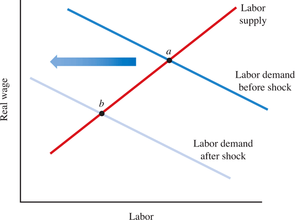
According to the Real Business Cycle Theory (RBC), the economy is constantly adjusting to technology shocks (e.g., an oil price shock) that keep hitting the economy. After a shock, the economy “swings” back to equilibrium. This interplay of shocks and the post-shock reaction of the economy causes fluctuations in GDP, employment, investment, etc.
9.4.1 RBC and Adverse Shock
An adverse shock to the economy (like an oil price shock) shifts the labor demand curve to the left. Think of this as a negative shock to TFP, the letter A in the production function discussed above. As TFP decreases, labor becomes less productive, so that firms start demanding less of it. The result is lower wages, reduced employment, and reduced output. The economy contracts (shrinks).
The key lesson from real business cycle theory is that potential output itself will vary over time, depending on the level of TFP.
9.4.2 Dividing Output Among Competing Demands
Together, labor and the supply of capital determine the level of output through the production function. This means that in a full-employment economy, total GDP is determined by the supply of factors of production.
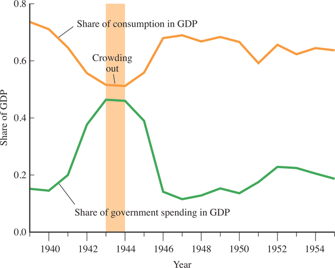
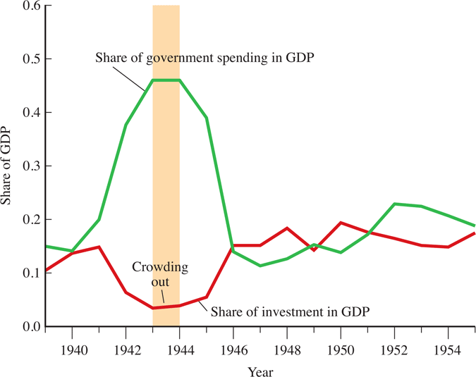
Full-employment GDP must be divided among competing demands in the economy. For example, increased government spending affects private spending (Crowding out).
Crowding Out
Increased government spending “crowds out” other demands for GDP.
Crowding out illustrates the principle of opportunity cost.
PRINCIPLE of Opportunity Cost
The opportunity cost of something is what you sacrifice to get it.
At full employment, the opportunity cost of increased government spending is some other component of GDP that needs to decrease in order to clear the accounting identity
\[Y = C + I + G + NX\]
- Crowding Out:
-
At full employment, that is Y is fixed, G increases, then either C, I, or NX or a combination of these decrease
- Crowding In:
-
G decreases, hence, C,I, or NX increase
9.4.3 Crowding Out in a Closed Economy
An economy without international trade is called a closed economy. In this economy, full-employment output is divided among three different demands:
\[Y=C+I+G\]
The supply of output (Y) is fixed. Therefore, increases in government spending reduce, or crowd out, either consumption or investment. In general, both are affected.
9.4.4 Crowding Out in an Open Economy
In an open economy, an economy with international trade, full-employment output is divided among four uses:
\[Y=C+I+G+NX\]
In an open economy, increases in government spending need not crowd out either consumption or investment. Increased government spending could lead to reduced exports and increased imports.
9.4.5 Crowding In
When governments cut spending and the level of output is fixed, some other type of spending will increase. We call this crowding in.
- In a closed economy, consumption or investment or both could increase.
- In an open economy, net exports could increase as well.
The nature of changes in government spending will have some effect on the type of spending that is crowded in (or crowded out)
- RBC theory studies the effects of technology shocks on the economy.
- Crowding out describes how an increase in government spending causes either private consumption, investment or net exports to decrease.
- Explain the concept of crowding-out.
- Explain the concept of crowding-in.
