17 From Short-Run to Long-Run
One of the great debates surrounding macroeconomic policymaking centers on the short run versus the long run. Up to this point, we have discussed the short and long run separately. Now, however, we explain how the economy evolves from the short run to the long run. The relationship between the two is one of the most important dimensions of modern macroeconomics, which carefully distinguishes between them.
We will next describe the differences between the short run and the long run. This discussion is then followed by explaining how the economy evolves from the short to the long run. We then discuss how monetary policy is neutral in the long run so that it does not have a 'real' effect. Finally we discuss the issue of crowding out.
17.1 The Difference Between the Short and Long Run
Earlier we explained how in the short run, wages and prices are sticky and do not change immediately in response to changes in demand. The short run in macroeconomics is the period of time over which prices do not change or do not change very much.
Short-run: Wages and prices are sticky
– Short-run analysis applies to the period of time when wages and prices do not change—at least not substantially
– The level of GDP is determined by the current demand for goods and services
– Monetary and fiscal policies can have an impact on demand and GDP
In the long run, GDP is determined by the current demand for goods and services in the economy, so fiscal policy---such as tax cuts or increased government spending--- and monetary policy---such as adjusting the money supply---can affect demand and GDP. However, in the long run, GDP is determined by the supply of labor, the stock of capital, and technological progress---in other words, the willingness of people to work and the overall resources the economy has to work with.
Long run: Prices are flexible
– The level of GDP is determined by the demand and supply for labor, the stock of capital, and technological progress
– The economy operates at full employment
– Output can’t be increased by changes in demand
– Any increases in government spending must come at the sacrifice of some other use of outputrightarrowcrowding-out
– An increase in the money supply will only cause the price level to riserightarrow neutrality of MP
17.1.1 Wage and Prices and Their Adjustment Over Time
Wages and prices change every day. If the demand for scooters rises at the same time that demand for tennis rackets falls, we would expect to see a rise in the price of scooters and a fall in the price of tennis rackets. Wages in the scooter industry would tend to increase, and wages in the tennis racket industry would tend to fall.
Sometimes, we see wages and prices in all industries rising of falling together. Why? Wages and prices will all tend to increase together during booms when GDP exceeds its full-employment level or potential output. Wages and prices will fall together during periods of recessions when GDP falls below full employment or potential output.
if the economy is producing at a level above full employment, firms will find it increasingly difficult to hire and retain workers, and unemployment will be below its natural rate. Workers will find it easy to get and changes jobs. To attract workers and prevent them from leaving, firms will raise their wages. As one firm raises its wage, other firms will have to raise their wages even higher to attract the workers that remain. Wages are the largest cost of production for most firms. Consequently, as labor costs increase, firms have no choice but to increase the prices of their products. However, as prices rise, workers need higher nominal wages to maintain their real wages.
\[\text{real-wage}=\frac{w}{P_{c}}\]
This is an illustration of the real-nominal principle:
What matters to people is the real value of money or income—its purchasing power—not the “face” value of money or income
This process by which rising wages cause higher prices and higher prices feed higher wages in known as the wage-price spiral.
A wage-price spiral occurs when actual output produced exceeds the potential output of the economy. When the economy is producing below full employment or potential output, the process works in reverse.
Table 17.1 summarizes the argument.
| When unemployment is below natural rate | When unemployment is above natural rate |
|---|---|
| output is above potential | output is below potential |
| wage and prices rise | wages and prices fall |
- In the short run wages and prices are sticky.
- In the long run wages and prices can adjust and are flexible.
- The process by which rising wages cause higher prices and higher prices feed higher wages in known as the wage-price spiral.
- Wages and prices will increase when actual output exceeds potential? (true/false)
- In the long run, the level of GDP is determined by demand factors (true/talse)
17.2 The Adjustment Process
The transition between the short run and the long run is easy to understand. If GDP is higher than potential output, the economy starts to overheat and wages and prices increases. This increase in wages and prices will then push the economy back to full employment. Using aggregate demand and aggregate supply, we can illustrate graphically how changing prices and wages help move the economy from the short to the long run. First, let's review the graphical representations of aggregate demand and aggregate supply:
Aggregate demand. Recall that the aggregate demand curve shows the relationship between the level of prices and the quantity of real GDP demanded.
Aggregate supply. Recall the there are two aggregate supply curves: - one for the short run and - one for the long run.
The short run aggregate supply curve is represented as a relatively flat curve. The shape of the curve reflects the idea that prices do not change very much in the short urn and that firms adjust production to meet demand.
The long run aggregate supply curve, however, is represented by a perfectly vertical line. The vertical line means that at any given price level, firms in the long run are producing all that they can, given the amount of labor, capital, and technology available to them in the economy. The line represents what firms can supply in the long run at a state of full employment or potential output.
17.2.1 Returning to Full Employment from a Bust
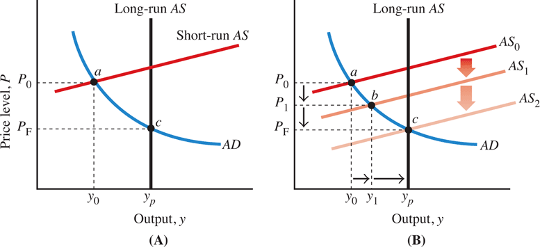
In an earlier chapter, we looked at the adjustment process for an economy producing at a level of output exceeding full employment or potential output. Now let’s look at what happens if the economy is in a slump, producing below full employment or potential output. Panel A of Figure 17.1 shows an aggregate demand curve and the two aggregate supply curves.
In the short run, output and prices are determined where the aggregate demand curve intersects the short-run aggregate supply curve—point \(a\). This point corresponds to the level of output \(y_0\) and a price level \(P_0\). Notice that \(y_0\) is a level less than full employment or potential output, \(y_p\).
In the long run, the level of prices and output is given by the intersection of the aggregate demand curve and the long-run aggregate supply curve—point \(c\). Output is at full employment, \(y_p\), and prices are at \(P_F\).
How does the economy move from point \(a\) in the short run to point \(c\) in the long run? Panel B of Figure 17.1 shows us how. At point \(a\), the current level of output, \(y0\), falls short of the full-employment level of output, \(y_p\). With output less than full employment, the unemployment rate is above the natural rate. Firms find it relatively easy to hire and retain workers, and wages and then prices begin to fall. As the level of prices decreases, the short-run aggregate supply curve shifts downward over time, as shown in Panel B.
This downward shift occurs because decreases in wages lower costs for firms. Competition between firms will lead to lower prices for their products. As shown in Panel B, this shift in the short-run aggregate supply curve will bring the economy to long-run equilibrium. The economy initially starts at point a, where output falls short of full employment. As prices fall from \(P_0\) to \(P_1\), the aggregate supply curve shifts downward from AS0 to AS1. The aggregate demand curve and the new aggregate supply curve intersect at point \(b\).
This point corresponds to a lower level of prices and a higher level of real output. However, the higher level of output still is less than full employment. Wages and prices will continue to fall, shifting the short-run aggregate supply curve downward. Eventually, the aggregate supply curve will shift to \(AS_2\), and the economy will reach point \(c\), the intersection of the aggregate demand curve and the long-run aggregate supply curve. At this point, the adjustment stops because the economy is at full employment and the unemployment rate is at the natural rate. With unemployment at the natural rate, the downward wage–price spiral ends. The economy has made the transition to the long run. Prices are lower and output returns to full employment. This is how an economy recovers from a recession or a downturn
How the Economy Recovers from a Downturn?
– If the economy is operating below full employment, as shown in Panel A, prices will fall, shifting down the short-run aggregate supply curve, as shown in Panel B.
– This will return output to its full-employment level
17.2.2 Returning to Full Employment from a Boom
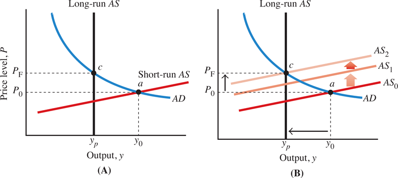
But what if the economy is “too hot” instead of sluggish? What will then happen is the process we just described, only in reverse, as we show in Figure 17.2. When output exceeds potential, unemployment will be below the natural rate. As firms bid for labor, the wage–price spiral will begin, but this time in an upward direction instead of downward as in Panel B. The short-run aggregate supply curve will shift upward until the economy returns to full employment. That is, wages and prices will rise to return the economy to its long-run equilibrium at full employment.
If the economy is operating above full employment, \(Y_{0}>Y_{F}\), as shown in Figure 17.2 Panel A, prices will rise, shifting the short-run aggregate supply curve upward, as shown in Panel B. This will return output to its full-employment level
In summary:
- – If output is less than full employment, prices will fall as the economy
-
returns to full employment as shown in Figure 17.1.
– If output exceeds full employment then
– Economy is overheating – Wages and prices rise – Higher price increases the demand for money – Interests rise and decrease investment – Which reduces the level of output back to full employment levels as shown in Figure 17.2
17.2.3 Details on the Adjustment Process
Earlier in the chapter we explained that changes in wages and prices restore the economy to full employment in the long run, and that the government and the Fed can get it there more quickly with fiscal and monetary policy. But what is happening behind the scenes? What do changes in wages and the price level mean for the economy in terms of money demand, interest rates, and investment spending? Let’s go back and take a closer look at the adjustment process in terms of these factors so we can better understand how the adjustment process actually works.
First, recall that when an economy is producing below full employment, the tendency will be for wages and prices to fall. Similarly, when an economy is producing at a level exceeding full employment or potential output, the tendency will be for wages and prices to rise.
The adjustment process first begins to work as changes in prices affect the demand for money. Recall the real-nominal principle.
Real-Nominal Principle
What matters to people is the real value of money or income—its purchasing power—not the face value of money or income.
According to this principle, the amount of money people want to hold depends on the price level in the economy. If prices are cut in half, you need to hold only half as much money to purchase the same goods and services. Decreases in the price level will cause the money demand curve to shift to the left; increases in the price level will shift it to the right. Now let’s put this idea to use.
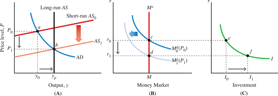
Suppose the economy is initially in a recession. With output below full employment, actual unemployment will exceed the natural rate of unemployment, so there will be excess unemployment. Wages and prices will start to fall. Figure 17.3 shows how the fall in the price level can restore the economy to full employment via money demand, interest rates, and investment without active fiscal or monetary policy. First, we show with the AD–AS diagram in Panel A of Figure 17.3 how prices fall when the economy is operating below full employment.
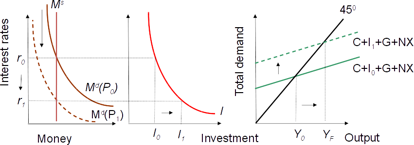
Second, in Panel B of Figure 17.3, the fall in the price level decreases the demand for holding money. As the price level decreases from \(P_0\) to \(P_1\), the demand for money shifts to the left from \(M^d_0\) to \(M^d_1\). Interest rates fall from \(r_0\) to \(r_1\), and the falling interest rates increase investment spending from \(I_0\) to \(I_1\). As the level of investment spending in the economy increases, total demand for goods and services also increases, and the economy moves down along the aggregate demand curve as it returns to full employment. Now you can also understand why the aggregate demand curve is downward sloping through the interest rate effect. As we move down the aggregate demand curve, lower prices lead to lower interest rates, higher investment spending, and a higher level of aggregate demand. Thus, aggregate demand increases as the price level falls, which explains why the curve slopes downward.
What we have just described continues until the economy reaches full employment. As long as actual output is below the economy’s full-employment level, prices will continue to fall. A fall in the price level reduces money demand and interest rates. Lower interest rates stimulate investment spending and push the economy back toward full employment. All this works in reverse if output exceeds the economy’s potential output. In this case, the economy is overheating and wages and prices rise. A higher price level will increase the demand for money and raise interest rates. Higher interest rates will decrease investment spending and reduce the level of output. The process continues until the economy “cools off” and returns to full employment.
Now you should understand why changes in wages and prices restore the economy to full employment. The key is that (1) changes in wages and prices change the demand for money, and (2) this changes interest rates, which then affect aggregate demand for goods and services and ultimately GDP.
Liquidity Trap
We can also use the model we just developed to understand the liquidity trap and the economics of the zero lower bound. If an economy is in a recession, interest rates will fall, restoring the economy to full employment. But at some point, interest rates may become so low they equal zero. Nominal interest rates cannot go far below zero because investors would rather hold money (which pays a zero rate) than hold a bond that promises a negative return.
Suppose, however, that as interest rates approach zero, the economy is still in a slump. The adjustment process then has nowhere to go. This appears to be what happened in Japan in the 1990s. Interest rates on government bonds were zero, but prices continued to fall. At this point, the fall in prices by itself could not restore the economy to full employment.
Policymakers in the United States also became concerned by this possibility. When interest rates on 3-month U.S. government bills fell below 1 percent from June 2003 to May 2004, Fed officials openly discussed their limited options if further monetary stimulus became necessary. What can policymakers do if an economy is in a recession but nominal rates become so close to zero that the natural adjustment process ceases to work? Economists have suggested several solutions to this problem.
First, expansionary fiscal policy— cutting taxes or raising government spending—still remains a viable option to increase aggregate demand.
Second, the Fed could become extremely aggressive and try to expand the money supply so rapidly that the public begins to anticipate future inflation. If the public expects inflation, the expected real rate of interest (the nominal rate minus the expected inflation rate) can become negative, even if the nominal rate cannot fall below zero. A negative expected real interest rate will tempt firms to invest, and this will increase aggregate demand.
In summary, the adjustment process works as follows:
With the economy initially below full employment, the price level falls, as shown in Panel A, stimulating output
In Panel B, the lower price level decreases the demand for money and leads to lower interest rates at point d
In Panel C, lower interest rates lead to higher investment spending at point f
As the economy moves down the AD curve from point a toward full employment at point b in Panel A, investment spending increases along the AD curve
The Connection with the Expenditure Model
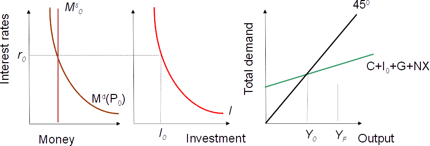
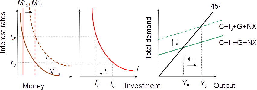
In Figure 17.4 and Figure 17.5 we also include the expenditure model graph so you can see how the mechanism works. In a Model of demand with money \(Y_{0}<Y_{F}\)
- Output \(Y_{0}\) is below full employment output \(Y_{F} \rightarrow\) excess unemployment
- Wages and prices will start to fall
- Fall in price level will decrease the demand for money and the \(M^{d}\) curve shifts to the left
- Interest rates fall and investment increases
- This increases the level of output
- This goes on until the economy reaches full employment again
17.3 How Economic Policy Can Hasten the Speed of Adjustment
How long does it take to move from the short run to the long run? Economists disagree on the answer. Some economists estimate it takes the U.S. economy 2 years or less, some say 6 years, and others say somewhere in between. Because the adjustment process is slow, there is room, in principle, for policymakers to step in and guide the economy back to full employment.
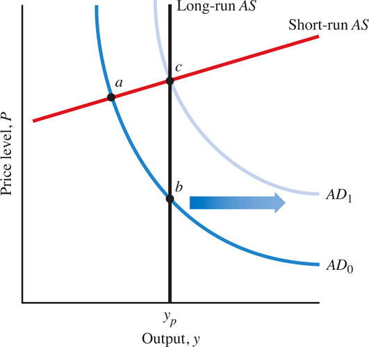
Suppose the economy is operating below full employment at point \(a\) in Figure 17.6. One alternative for policymakers is to do nothing, allowing the economy to adjust itself with falling wages and prices until it returns by itself to full employment, point \(b\). This may take several years. During that time, the economy will experience excess unemployment and a level of real output below potential.
Another alternative is to use expansionary policies, such as open market purchases (of bonds) by the Fed or increases in government spending and tax cuts, to shift the aggregate demand curve to the right.
IORB rate is the new monetary policy tool since 2020!
Keep in mind that since 2020 the Fed pays interest on bank reserves and uses that Interest on Bank Reserves (IORB) rate as the new monetary policy tool. Expansionary monetary policy would mean that the Fed lowers the IORB rate. This reduces the amount of reserves held with the central bank and private banks have more funds to give out loans, which expands money supply.
In Figure 17.6, we show how expansionary policies could shift the aggregate demand curve from \(AD_0\) to \(AD_1\) and move the economy to full employment, point \(c\). Notice here that the price level is higher at point \(c\) than it would be at point \(b\).
Demand policies can also prevent a wage–price spiral from emerging if the economy is producing at a level of output above full employment. Rather than letting an increase in wages and prices bring the economy back to full employment, we can reduce aggregate demand.
Either contractionary monetary policy—open-market sales—or contractionary fiscal policy—cuts in government spending or tax increases—can be used to reduce aggregate demand and the level of GDP until it reaches potential output.
Expansionary policies and demand policies are stabilization policies, which look simple on paper or on graphs. In practice, the lags and uncertainties we discussed for both fiscal and monetary policy make economic stabilization difficult to achieve.
For example, suppose we are in a recession and the Fed decides to increase aggregate demand using expansionary monetary policy. There will be a lag in the time it takes for the aggregate demand curve to shift to the right. In the meantime, the adjustment that occurs during a recession—falling wages and prices—has begun to shift the short-run aggregate supply curve downward.
It is conceivable that if the adjustment were fast enough, the economy would be restored to full employment before the effects of the expansionary monetary policy were actually felt. When the expansionary monetary policy kicks in and the aggregate demand curve finally shifts to the right, the additional aggregate demand would increase the level of output so it exceeded the full-employment level, leading to a wage–price spiral.
In this case, monetary policy would have destabilized the economy. Active economic policies are more likely to destabilize the economy if the adjustment is quick enough. Economists like Milton Friedman (1912–2006) of the University of Chicago believed the economy adjusts rapidly to full employment and generally opposed using monetary or fiscal policy to try to stabilize the economy. Economists like John Maynard Keynes believed that the economy adjusted slowly and were more sympathetic to using monetary or fiscal policy to stabilize the economy. It is possible that the speed of adjustment can vary over time, making decisions about policy even more difficult.
As an example, economic advisers for President George H. W. Bush had to decide whether the economy needed any additional stimulus after the recession of 1990. Based on the view that the economy would recover quickly on its own, they took only some minor steps. The economy did largely recover by the very end of the Bush administration, but too late for his reelection prospects.
17.3.1 Liquidity Traps
Up to this point, we have assumed the economy could always recover from a recession without active policy, although it may take a long time. Economist John Maynard Keynes expressed doubts about whether a country could recover from a major recession without active policy. He had two distinct reasons for these doubts.
First, as we discuss later in the chapter, the adjustment process requires interest rates to fall and thereby increase investment spending. But suppose nominal interest rates become so low that they could not fall any further. Keynes called this situation a liquidity trap. Today, this is known as the zero lower bound for interest rates—that is, they cannot fall below zero. When the economy is experiencing a liquidity trap or the zero lower bound, the adjustment process no longer works.
Second, Keynes feared falling prices could hurt businesses (i.e., more difficult to repay debt). Japan seems to have suffered from both these problems in the 1990s and the United States faced similar issues during the first decade of this century.
Expansionary fiscal policy could still work
Fed could become very aggressive and expand money supply rapidly to generate expected inflation rightarrowcould turn real interest rate negative rightarrow stimulate investment
- Recall that the aggregate demand curve represents the total demand for all currently produced goods and services at different price levels
- The short-run aggregate supply curve is represented as a relatively flat curve that reflects the idea that prices do not change very much in the short run and that firms adjust production to meet demand
- The long-run aggregate supply curve is represented by a perfectly vertical line at the full-employment level of output
- Rather than letting the economy naturally return to full employment, economic policies could be implemented to increase aggregate demand to bring the economy to full employment faster. The price level within the economy, however, would be higher.
- Liquidity trap \(\rightarrow\) a situation in which nominal interest rates are so low, they can no longer fall
- What would be your policy recommendation if the economy is in a liquidity trap?
- What policy would you recommend if the economy is overheating?
17.4 The Long-Run Neutrality of Money
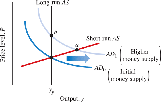
An increase in the money supply has a different effect on the economy in the short run than it does in the long run. In Figure 17.7, we show the effects of expansionary monetary policy in both the short run and the long run. In the short run, as the supply of money increases, the economy moves from the original equilibrium to point a, with output above potential. But in the long run, the economy returns to point \(b\) at full employment, but at a higher price level than at the original equilibrium.
How can the Federal Reserve change the level of output in the short run but affect prices only in the long run? Why is the short run different from the long run? We can use our model of the demand for money and investment to understand this issue.
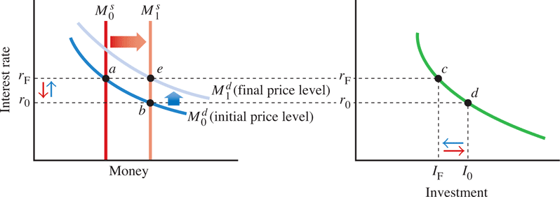
Assume the economy starts at full employment. In Figure 17.8, interest rates are at \(r_F\), and investment spending is at \(I_F\). Now, suppose the Federal Reserve increases the money supply from \(M^s_0\) to \(M^s_1\). We show this as a rightward movement in the money-supply curve. In the short run, the increase in the supply of money will reduce interest rates to \(r_0\), and the level of investment spending will increase to \(I_0\). Increased investment will stimulate the economy and increase output above full employment. All this occurs in the short run. The red arrows show the movements in interest rates and investment in the short run. However, once output exceeds full employment, wages and prices will start to increase. As the price level increases, the demand for money will increase. This will shift the money-demand curve upward and will start to increase interest rates. Investment will start to fall as interest rates increase, leading to a fall in output. The blue arrows in Figure 17.8 show the transition as prices increase.
As long as output exceeds full employment, prices will continue to rise, money demand will continue to increase, and interest rates will continue to rise. Where does this process end? It ends only when interest rates return to their original level of \(r_F\).
At an interest rate of \(r_F\), investment spending will have returned to \(I_F\). This is the level of investment that meets the total level of demand for goods and services and keeps the economy at full employment. When the economy returns to full employment, the levels of real interest rates, investment, and output are precisely the same as they were before the Fed increased the supply of money. The increase in the supply of money had no effect on real interest rates, investment, or output in the long run. Economists call this the long-run neutrality of money. In other words, in the long run, changes in the supply of money are neutral with respect to real variables in the economy. For example, if the price of everything in the economy doubles, including your paycheck, you are no better or worse off than you were before. In the long run, increases in the supply of money have no effect on real variables, only on prices.
This example points out how, in the long run, it really does not matter how much money is in circulation because prices will adjust to the amount of nominal money available. In the short run, however, money is not neutral. In the short run, changes in the supply of money do affect interest rates, investment spending, and output. The Fed does have strong powers over real GDP, but those powers are ultimately temporary. In the long run, all the Fed can do is determine the level of prices in the economy.
Now we can understand why the job of the Federal Reserve has been described by William McChesney Martin, Jr., a former Federal Reserve chairman, as “taking the punch bowl away at the party.” The punch bowl is money: If the Fed sets out the punch bowl, this will temporarily increase output or give the economy a brief high. But if the Federal Reserve is worried about increases in prices in the long run, it must take the punch bowl away and everyone must sober up. If not, the result will be continuing increases in prices, or inflation.
Let's summarize the adjustment processes:
- Fed increases \(M^{s}, M^{d}\) adjusts, prices rise and GDP stays constant
- As the Fed increases the supply of money, the aggregate demand curve shifts from \(AD_{0}\) to \(AD_{1}\)
- In the long run, the economy returns to long-run equilibrium
In more detail:
Starting at full employment, an increase in the supply of money from \(M_{0}^{s}\) to \(M_{1}^{s}\) will initially
reduce interest rates from \(r_{F}\) to \(r_{0} \rightarrow\) point a to point b and
raise investment spending from \(I_{_{F}}\) to \(I_{0} \rightarrow\) point c to point d
We show these changes with the red arrows in Figure 17.8.
The blue arrows in Figure 17.8 show that as the price level increases, the demand for money increases, restoring interest rates and investment to their prior levels—\(r_{F}\) and \(I_{F}\), respectively
Both money supplied and money demanded will remain at a higher level, though, at point e in Figure 17.8.
Money is NOT Neutral in the Short Run.
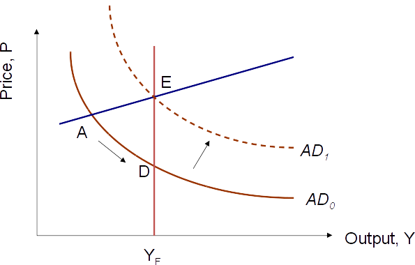
In the short run, monetary policy is not neutral. Let us start with an economy in a recession as in point A of Figure 17.10.
An increase in the money supply would decrease the interest rate, therefore increase investment and subsequently output, so that aggregate demand would shift to the right.
The price level would still increase, but the economy has moved back to full employment.
- Monetary policy is neutral in the long run, i.e., it will not affect output.
- Monetary policy is non-netural in the short run, i.e., expansionary monetary policy stimulates the economy and increases aggregate demand.
- What happens to output and prices in the long run if the FED conducts an open market purchase
- What happens to output and prices in the short run if the FED conducts an open market sale?
17.5 Short-Run vs Long-Run Debate
Short Run
- Money is NOT neutral in the short run
- The Fed can influence the level of real GDP in the short run
- However, this power is only temporary
- Short run is 2 to 6 years
17.5.1 “Classical Economics” in Historical Perspective
The term classical economics refers to the work of the originators of modern economic thought. Adam Smith was the first so-called classical economist. Other classical economists—Jean-Baptiste Say, David Ricardo, John Stuart Mill, and Thomas Malthus—developed their work during the late eighteenth and nineteenth centuries. Keynes first used the term classical model in the 1930s to contrast it with his Keynesian model, which emphasized the difficulties the economy could face in the short run. The ideas developed in this chapter can shed some light on a historical debate in economics about the role of full employment in modern Keynesian and classical thought.
- The term “classical model” was first used by Keynes to contrast his “Keynesian” or activist model with the conventional economic wisdom of the time that didn’t emphasize the difficulties that the economy could face in the short run
Classical economics is often associated with Say’s law, the doctrine that “supply creates its own demand.” To understand Say’s law, recall from our discussion of GDP accounting in Chapter 5 that production in an economy creates an equivalent amount of income. For example, if GDP is $10 trillion, then production is $10 trillion, and $10 trillion in income is generated. The classical economists argued that the $10 trillion of production also created $10 trillion in demand for current goods and services. This meant there could never be a shortage of demand for total goods and services in the economy, nor any excess.
“supply creates its own demand.”
But suppose consumers, who earned the income, decided to save rather than spend it. Wouldn’t this increase in saving lead to a shortfall in the total demand for goods and services? Wouldn’t, say, inventories of goods pile up in warehouses? Classical economists argued no, that the increase in savings would eventually find its way to an equivalent increase in investment spending by firms because the savings by households would eventually get channeled to firms via financial markets. As a result, spending on consumption and investment together would be sufficient so that all the goods and services produced in the economy would be purchased.
Keynes, on the other hand, argued that there could be situations in which total demand fell short of total production in the economy for extended periods of time. In particular, if consumers increased their savings, there was no guarantee that investment spending would rise to offset the decrease in consumption. And if total spending did fall short of total demand, goods and services would go unsold. When producers could not sell their goods, they would cut back on production, and output in the economy would consequently fall, leading to a recession or depression.
In summary:
Since production creates an equivalent amount of income, there could never be a shortage of demand for total goods and services in the economy nor any excess
If consumers saved, those savings would eventually turn into investment spending
Keynes argued that there could be situations in which total demand fell short of total production in the economy, leading to a recession or depression
– If wages and prices are not fully flexible, then Keynes’s view that demand could fall short of production is more likely to hold true
– However, over longer periods of time, wages and prices do adjust and the insights of the classical model are restored
Keynesian and Classical Debates
The debates between Keynesian and classical economists continued for several decades after Keynes developed his theories. In the 1940s, Professor Don Patinkin and Nobel Laureate Franco Modigliani clarified the conditions for which the classical model would hold true. In particular, they studied the conditions under which there would be sufficient demand for goods and services when the economy was at full employment. Both economists emphasized that one of the necessary conditions for the classical model to work was that wages and prices must be fully flexible—that is, they must adjust rapidly to changes in demand and supply.
If wages and prices are not fully flexible, then Keynes’s view that demand could fall short of production is more likely to hold true. We’ve seen that over short periods of time, wages and prices, indeed, are not fully flexible, so Keynes’s insights are important. However, over longer periods of time, wages and prices do adjust and the insights of the classical model are restored.
To help clarify the conditions under which the economy will return to full employment in the long run on its own, Patinkin and Modigliani developed the adjustmentprocess model we used in this chapter. They highlighted many of the key points we emphasized, including the speed of the adjustment process and possible pitfalls, such as liquidity traps.
17.5.2 Speed of Adjustment and Keynes' Ideas
How long does it take to move from the short run to the long run? Economists disagree on the answer. Some economists estimate it takes the U.S. economy 2 years or less, some say 6 years, and others say somewhere in between. Because the adjustment process is slow, there is room, in principle, for policymakers to step in and guide the economy back to full employment.
Suppose the economy is operating below full employment at point a in Figure 17.11. One alternative for policymakers is to do nothing, allowing the economy to adjust itself with falling wages and prices until it returns by itself to full employment, point b. This may take several years. During that time, the economy will experience excess unemployment and a level of real output below potential. Another alternative is to use expansionary policies, such as open market purchases by the Fed or increases in government spending and tax cuts, to shift the aggregate demand curve to the right.
In Figure 17.11, we show how expansionary policies could shift the aggregate demand curve from \(AD_0\) to \(AD_1\) and move the economy to full employment, point \(c\). Notice here that the price level is higher at point \(c\) than it would be at point \(b\).
Demand policies can also prevent a wage–price spiral from emerging if the economy is producing at a level of output above full employment. Rather than letting an increase in wages and prices bring the economy back to full employment, we can reduce aggregate demand. Either
contractionary monetary policy—open-market sales—or
contractionary fiscal policy—cuts in government spending or tax increases
can be used to reduce aggregate demand and the level of GDP until it reaches potential output.
Expansionary policies and demand policies are stabilization policies, which look simple on paper or on graphs. In practice, the lags and uncertainties we discussed for both fiscal and monetary policy make economic stabilization difficult to achieve. For example, suppose we are in a recession and the Fed decides to increase aggregate demand using expansionary monetary policy. There will be a lag in the time it takes for the aggregate demand curve to shift to the right. In the meantime, the adjustment that occurs during a recession—falling wages and prices—has begun to shift the short-run aggregate supply curve downward.
It is conceivable that if the adjustment were fast enough, the economy would be restored to full employment before the effects of the expansionary monetary policy were actually felt. When the expansionary monetary policy kicks in and the aggregate demand curve finally shifts to the right, the additional aggregate demand would increase the level of output so it exceeded the full-employment level, leading to a wage–price spiral. In this case, monetary policy would have destabilized the economy.
Active economic policies are more likely to destabilize the economy if the adjustment is quick enough. Economists like Milton Friedman (1912–2006) of the University of Chicago believed the economy adjusts rapidly to full employment and generally opposed using monetary or fiscal policy to try to stabilize the economy. Economists like John Maynard Keynes believed that the economy adjusted slowly and were more sympathetic to using monetary or fiscal policy to stabilize the economy.
It is possible that the speed of adjustment can vary over time, making decisions about policy even more difficult. As an example, economic advisers for President George H. W. Bush had to decide whether the economy needed any additional stimulus after the recession of 1990. Based on the view that the economy would recover quickly on its own, they took only some minor steps. The economy did largely recover by the very end of the Bush administration, but too late for his reelection prospects.
How long does it take to move from the short run to the long run?
Estimates range from 2 to 6 years!
Keynes or Not Keynes?
- We are at A
- Do nothing and wait till D
- Or do Keynesian expansionary policy and get to E
Is it a Question of Believe?
- Some economists think that the economy adjusts quickly to the full employment level and that fiscal or monetary policy destabilize the economy (classical approach)
- So the long run is actually quite short
- Others believe that the economy is slow to adjust and hence monetary or fiscal policy make sense (Keynesian view)
- In the long run we are all dead (according to Keynes)
- That’s how long the long run is!
- What would a classical economist prescribe during a recession?
- What would a Keynesian economist prescribe during a boom?
17.6 Political Economy Considerations
Some economists are strong proponents of increasing government spending on defense or other programs to stimulate the economy. Critics, however, say increases in spending provide only temporary relief and ultimately harm the economy because government spending crowds out investment spending. In an earlier chapter, we discussed the idea of crowding out. We can now understand the idea in more detail. Suppose the economy starts out at full employment and then the government increases its spending. This will shift the aggregate demand curve to the right, causing output to increase beyond full employment. As we have seen, the result of this boom will be that wages and prices increase.
17.6.1 Crowding Out
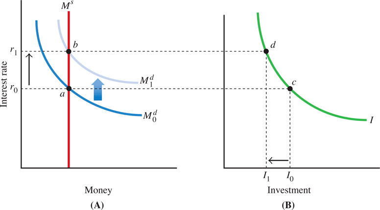
Now let’s turn to our model of money demand and investment. Figure 17.13 shows that as prices increase, the demand for money shifts upward in Panel A, raising interest rates from \(r_0\) to \(r_1\) and reducing investment from \(I_0\) to \(I_1\), as shown in Panel B.
Higher interest rates are the mechanism through which crowding out of public investment occurs. As investment spending by the public then falls (gets crowded out), we know that aggregate demand decreases. This process will continue until the economy returns to full employment. Once the economy returns to full employment, the decrease in investment spending by the public will exactly match the increase in government spending.
However, when the economy does return to full employment, it will be at a higher interest rate level and lower level of investment spending by the public. Thus, the increase in government spending has no long-run effect on the level of output—just on the interest rate. Instead, the increase in government spending displaced, or crowded out, private investment spending. If the government spending went toward government investment projects—such as bridges or roads—then it will have just replaced an equivalent amount of private investment. If the increased government spending did not go toward providing investment but, for example, went for military spending, then the reduction in private investment will have reduced total investment in the economy, private and public. This decrease in total investment would have further negative effects on the economy over time. As we saw in earlier chapters, a reduction in investment spending reduces capital deepening and leads to lower levels of real income and wages in the future.
Economists make similar arguments when it comes to tax cuts. Tax cuts initially will increase consumer spending and lead to a higher level of GDP. In the long run, however, adjustments in wages and prices restore the economy to full employment. However, interest rates will rise during the adjustment process and this increase in interest rates will crowd out private investment. In the long run, the increase in consumption spending will come at the expense of lower investment spending, decreased capital deepening, and lower levels of real income and wages in the future. Crowding out can occur from sources other than the government. Expected increases in U.S. health-care expenditures will pose similar challenges to crowding out in the coming decades as well.
What about decreases in government spending or increases in taxes? Decreases in government spending, such as cuts in military spending, will lead to increases in investment in the long run, which we call crowding in. Initially, a decrease in government spending will cause a decrease in real GDP. But as prices fall, the demand for money will decrease, and interest rates will fall. Lower interest rates will crowd in investment as the economy returns to full employment. In the longer run, the higher investment spending will raise living standards through capital deepening. Increased taxes, to the extent they reduce consumption spending, will crowd in investment through precisely the same mechanism.
Crowding Out Summary
Keynes claims that increases in G, stimulates the economy
Critics say, that this works only temporarily and ultimately harms the economy because G will crowd out investment spending
Starting at full employment, an increase in government spending G raises output above full employment
As wages and prices increase,
the demand for money increases, as shown in Panel A of Figure 17.13
raising interest rates from \(r_0\) to \(r_1 \rightarrow\) point \(a\) to point \(b\) and
reducing investment from \(I_0\) to \(I_1 \rightarrow\) point \(c\) to point \(d\)
Hence an increase of \(G\) decreased \(I\) and \(Y\) stayed constant in the long run
The economy returns to full employment, but at a higher level of interest rates and a lower level of investment spending
In the previous illustration, a long run increase in government spending has no long-run effect on the level of output—just the interest rate
Instead, the increase in government spending displaced, or crowded out, private investment spending
Example
In 1950, health-care expenditures in the United States were 5.2 percent of GDP; by 2000, this share had risen to 15.4 percent
Since 1950, the average life span has increased by 1.7 years per decade
Two economists, Charles I. Jones and Robert E. Hall, go further and suggest normal increases in economic growth will propel health-care expenditures to approximately 30 percent of GDP by mid-century
Their argument is that as societies grow wealthier, individuals face the trade-off of buying more goods (automobiles or cars) to enjoy their current life span or spending more on healthcare to extend their lives
Assuming this argument is correct and health-care expenditures increase, what other component of GDP will fall?
If investment is crowded out, living standards would fall in the long-run, reducing the ability to consume both health and non-health goods
Spending on health would then come at the expense of spending on consumer durables or larger houses. That would be the preferred outcome
17.6.2 Tax Cuts
Tax cuts may initially increase consumer spending and lead to a higher levels of GDP (expansionary fiscal policy). However, in the long run adjustments in wages and prices restore the economy to full employment output.
- Interest rates will rise during the adjustment process and crowd out investment
- Wages and prices will fall again
Crowding In
- Cuts in G (like cuts in military spending) will lead to increases in investment in the long run
- Initially though a decrease in G will cause a decrease in real GDP
- As prices fall interest go down \(\rightarrow\) and I goes up
17.6.3 Political Business Cycles
Up to now, we have assumed policymakers are motivated to use policy to try to improve the economy. But suppose they are more interested in promoting their personal wellbeing and the fortunes of their political parties? Using monetary or fiscal policy in the short run to improve a politician’s reelection prospects may generate what is known as a political business cycle.
Here is how a political business cycle might work. About a year or so before an election, a politician might use expansionary monetary policy or fiscal policy to stimulate the economy and lower unemployment. If voters respond favorably to lower unemployment, the incumbent politician may be reelected. After reelection, the politician faces the prospect of higher prices or crowding out. To avoid this, the politician may engage in contractionary policies. The result is a classic political business cycle: Because of actions taken by politicians for reelection, the economy booms before an election but contracts afterward. Good news comes before the election, and bad news comes later. It is clear the classic political business cycle does not always occur; however, a number of episodes fit the scenario. President Richard Nixon used expansionary policies during a reelection campaign in 1972, which resulted in inflation. However, counterexamples also exist, such as President Jimmy Carter’s deliberate attempt to reduce inflation with contractionary policies just before his reelection bid in the late 1970s.
Although the evidence on the classic political business cycle is mixed, there may be links between elections and economic outcomes. More recent research has investigated the systematic differences that may exist between political parties and economic outcomes. All this research takes into account both the short- and long-run effects of economic policies.
In Summary:
Using monetary and fiscal policy in the short run to improve a politician’s reelection prospects may generate what is known as a political business cycle
In a classic political business cycle, the economy booms before an election but then contracts after the election
The original political business cycle theories focused on incumbent presidents trying to manipulate the economy in their favor to gain reelection
Subsequent research began to incorporate other, more realistic factors:
The first innovation was to recognize that political parties could have different goals or preferences
Republicans historically have been more concerned about fighting inflation, whereas Democrats have placed more weight on reducing unemployment
The second major innovation was to recognize that the public would anticipate that politicians will try to manipulate the economy
If the public is not sure who will win the election, the outcome will be a surprise to them—a contractionary surprise if Republicans win and an expansionary surprise if Democrats win
This suggests that economic growth should be less if Republicans win and greater if Democrats win
The postwar U.S. evidence is generally supportive of this theory
- Crowding out refers to a situation where government spending (or consumption) leads to a reduction in personal consumption, investments and savings because the government is sucking up the available resources.
- Increases in government spending will raise real interest rates and crowd out investment in the long run. Decreases in government spending will lower real interest rates and crowd in investment in the long run.
- The adjustment model in this chapter helps us to understand the debate between Keynes and the classical economists.
- Using monetary and fiscal policy in the short run to improve a politician’s reelection prospects may generate what is known as a political business cycle
- Tax Increases and Crowding In. Using an aggregate demand and aggregate supply graph, show how tax increases for consumers today will eventually lead to lower interest rates and crowd in investment spending in the long run.
- Effects of Cross-Border Conflicts. Suppose that due to cross-border conflicts in an economy, domestic firms export less in order to meet the higher domestic consumption of goods. At the same time, the import of foreign goods increases. Assuming that the economy is initially at full employment and the exchange rate remains constant, what happens to the GDP in the short run and the long run?
