12 Government Budgets and Fiscal Policy
All levels of government—federal, state, and local—have budgets that show how much revenue the government expects to receive in taxes and other income and how the government plans to spend it. Budgets, however, can shift dramatically within a few years, as policy decisions and unexpected events disrupt earlier tax and spending plans.
In this chapter, we revisit fiscal policy, which we first covered in Welcome to Economics! Fiscal policy is one of two policy tools for fine tuning the economy (the other is monetary policy). While policymakers at the Federal Reserve make monetary policy, Congress and the President make fiscal policy.
The discussion of fiscal policy focuses on how federal government taxing and spending affects aggregate demand. All government spending and taxes affect the economy, but fiscal policy focuses strictly on federal government policies. We begin with an overview of U.S. government spending and taxes. We then discuss fiscal policy from a short-run perspective; that is, how government uses tax and spending policies to address recession, unemployment, and inflation; how periods of recession and growth affect government budgets; and the merits of balanced budget proposals.
NO YELLOWSTONE PARK?
You had trekked all the way to see Yellowstone National Park in the beautiful month of October 2013, only to find it… closed. Closed! Why?
For two weeks in October 2013, the U.S. federal government shut down. Many federal services, like the national parks, closed and 800,000 federal employees were furloughed. Tourists were shocked and so was the rest of the world: Congress and the President could not agree on a budget. Inside the Capitol, Republicans and Democrats argued about spending priorities and whether to increase the national debt limit. Each year's budget, which is over $3 trillion of spending, must be approved by Congress and signed by the President.
Two thirds of the budget are entitlements and other mandatory spending which occur without congressional or presidential action once the programs are established.
- Important entitlement programs are:
-
- Medicare (healthcare for the old),
- Medicaid (healthcare for the poor) and
- Social Security (pension payments to the old).
Tied to the budget debate was the issue of increasing the debt ceiling—how high the U.S. government's national debt can be. The House of Representatives refused to sign on to the bills to fund the government unless they included provisions to stop or change the Affordable Health Care Act (more colloquially known as Obamacare). As the days progressed, the United States came very close to defaulting on its debt.
Why does the federal budget create such intense debates? What would happen if the United States actually defaulted on its debt? In this chapter, we will examine the federal budget, taxation, and fiscal policy. We will also look at the annual federal budget deficits and the national debt.
12.1 Government Spending
Government spending covers a range of services that the federal, state, and local governments provide. When the federal government spends more money than it receives in taxes in a given year, it runs a budget deficit. Conversely, when the government receives more money in taxes than it spends in a year, it runs a budget surplus. If government spending and taxes are equal, it has a balanced budget. For example, in 2009, the U.S. government experienced its largest budget deficit ever, as the federal government spent $1.4 trillion more than it collected in taxes. This deficit was about 10% of the size of the U.S. GDP in 2009, making it by far the largest budget deficit relative to GDP since the mammoth borrowing the government used to finance World War II.
This section presents an overview of government spending in the United States.
12.1.1 Total U.S. Government Spending
Federal spending in nominal dollars (that is, dollars not adjusted for inflation) has grown by a multiple of more than 38 over the last four decades, from $93.4 billion in 1960 to $3.9 trillion in 2014. Comparing spending over time in nominal dollars is misleading because it does not take into account inflation or growth in population and the real economy. A more useful method of comparison is to examine government spending as a percent of GDP over time.
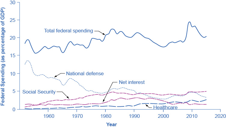
The top line in Figure 12.2 shows the federal spending level since 1960, expressed as a share of GDP. Despite a widespread sense among many Americans that the federal government has been growing steadily larger, the graph shows that federal spending has hovered in a range from 18% to 22% of GDP most of the time since 1960.
The other lines in Figure 12.2 show the major federal spending categories: national defense, Social Security, health programs, and interest payments. From the graph, we see that national defense spending as a share of GDP has generally declined since the 1960s, although there were some upward bumps in the 1980s buildup under President Ronald Reagan and in the aftermath of the terrorist attacks on September 11, 2001. In contrast, Social Security and healthcare have grown steadily as a percent of GDP. Healthcare expenditures include both payments for senior citizens (Medicare), and payments for low-income Americans (Medicaid). State governments also partially fund Medicaid. Interest payments are the final main category of government spending in Figure 12.2.
The graph shows five lines that represent different government spending from 1960 to 2014. Total federal spending has always remained above 17%. National defense has never risen above 10% and is currently closer to 5%. Social security has never risen above 5%. Net interest has always remained below 5%. Health is the only line on the graph that has primarily increased since 1960 when it was below 1% to 2014 when it was closer to 4%.
We broadly distinguish two types of programs in the government budget:
- entitlement programs or mandatory spending and
- discretionary spending programs.
As mentioned in the introduction, spending through entitlement programs occurs without congressional or presidential action once the programs are established. Important entitlement programs are:
- Medicare (healthcare for the old),
- Medicaid (healthcare for the poor) and
- Social Security (pension payments to the old).
Two thirds of the federal budget are entitlements and other mandatory spending. In order to change entitlement program spending, a law has to be passed. Because of this, changing entitlement program spending is very difficult.
Discretionary spending programs on the other hand can be changed by the administration on an annual basis (e.g., military spending) without changing a law and are thus easier to adjust.
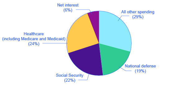
These four categories—national defense, Social Security, healthcare, and interest payments—account for roughly 73% of all federal spending, as Figure 12.3 shows. The remaining 27% wedge of the pie chart covers all other categories of federal government spending: international affairs; science and technology; natural resources and the environment; transportation; housing; education; income support for the poor; community and regional development; law enforcement and the judicial system; and the administrative costs of running the government.
The pie chart shows that healthcare (including Medicaid) makes up roughly 26% of federal spending; Social Security makes up 24%; national defense makes up 17%; net interest makes up over 6%; and all other spending makes up over 25%.
Each year, the government borrows funds from U.S. citizens and foreigners to cover its budget deficits. It does this by selling securities (Treasury bonds, notes, and bills)—in essence borrowing from the public and promising to repay with interest in the future. From 1961 to 1997, the U.S. government has run budget deficits, and thus borrowed funds, in almost every year. It had budget surpluses from 1998 to 2001, and then returned to deficits.
The interest payments on past federal government borrowing were typically 1–2% of GDP in the 1960s and 1970s but then climbed above 3% of GDP in the 1980s and stayed there until the late 1990s. The government was able to repay some of its past borrowing by running surpluses from 1998 to 2001 and, with help from low interest rates, the interest payments on past federal government borrowing had fallen back to 1.4% of GDP by 2012.
We investigate the government borrowing and debt patterns in more detail later in this chapter, but first we need to clarify the difference between the deficit and the debt. The deficit is not the debt. The difference between the deficit and the debt lies in the time frame.
- The government deficit (or surplus) refers to what happens with the federal government budget each year.
- The government debt is accumulated over time. It is the sum of all past deficits and surpluses.
If you borrow $10,000 per year for each of the four years of college, you might say that your annual deficit was $10,000, but your accumulated debt over the four years is $40,000.
12.1.2 State and Local Government Spending
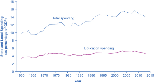
Although federal government spending often gets most of the media attention, state and local government spending is also substantial—at about $3.1 trillion in 2014. Figure 12.4 shows that state and local government spending has increased during the last four decades from around 8% to around 14% today.
The single biggest item is education, which accounts for about one-third of the total. The rest covers programs like highways, libraries, hospitals and healthcare, parks, and police and fire protection. Unlike the federal government, all states (except Vermont) have balanced budget laws, which means any gaps between revenues and spending must be closed by higher taxes, lower spending, drawing down their previous savings, or some combination of all of these.
The graph shows total state and local spending (as a percentage of GDP) was around 10% in 1960, and over 14% in 2013. Education spending at the state and local levels has risen minimally since 1960 when it was under 4% to more recently when it was closer to 4.5% in 2013.
U.S. presidential candidates often run for office pledging to improve the public schools or to get tough on crime. However, in the U.S. government system, these tasks are primarily state and local government responsibilities. In fiscal year 2014 state and local governments spent about $840 billion per year on education (including K–12 and college and university education), compared to only $100 billion by the federal government, according to usgovernmentspending.com. In other words, about 90 cents of every dollar spent on education happens at the state and local level. A politician who really wants hands-on responsibility for reforming education or reducing crime might do better to run for mayor of a large city or for state governor rather than for president of the United States.
- Fiscal policy is the set of policies that relate to federal government spending, taxation, and borrowing.
- In recent decades, the level of federal government spending and taxes, expressed as a share of GDP, has not changed much, typically fluctuating between about 18% to 22% of GDP.
- We distinguish between entitlement programs and discretionary spending programs.
- However, the level of state spending and taxes, as a share of GDP, has risen from about 12–13% to about 20% of GDP over the last four decades.
- The four main areas of federal spending are national defense, Social Security, healthcare, and interest payments, which together account for about 70% of all federal spending.
- When a government spends more than it collects in taxes, it is said to have a budget deficit.
- When a government collects more in taxes than it spends, it is said to have a budget surplus.
- If government spending and taxes are equal, it is said to have a balanced budget.
- The sum of all past deficits and surpluses make up the government debt.
- When governments run budget deficits, how do they make up the differences between tax revenue and spending?
- When governments run budget surpluses, what is done with the extra funds?
- Is it possible for a nation to run budget deficits and still have its debt/GDP ratio fall? Explain your answer. Is it possible for a nation to run budget surpluses and still have its debt/GDP ratio rise? Explain your answer.
- Give some examples of changes in federal spending and taxes by the government that would be fiscal policy and some that would not.
- Have the spending and taxes of the U.S. federal government generally had an upward or a downward trend in the last few decades?
- What are the main categories of U.S. federal government spending?
- What is the difference between a budget deficit, a balanced budget, and a budget surplus?
- Have spending and taxes by state and local governments in the United States had a generally upward or downward trend in the last few decades?
- Why is government spending typically measured as a percentage of GDP rather than in nominal dollars?
- Why are expenditures such as crime prevention and education typically done at the state and local level rather than at the federal level?
- Why is spending by the U.S. government on scientific research at NASA fiscal policy while spending by the University of Illinois is not fiscal policy? Why is a cut in the payroll tax fiscal policy whereas a cut in a state income tax is not fiscal policy?
12.2 Taxation
There are two main categories of taxes: those that the federal government collects and those that the state and local governments collect. What percentage the government collects and for what it uses that revenue varies greatly. The following sections will briefly explain the taxation system in the United States.
12.2.1 Federal Taxes
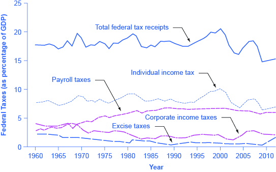
Just as many Americans erroneously think that federal spending has grown considerably, many also believe that taxes have increased substantially. The top line of Figure 12.5 shows total federal taxes as a share of GDP since 1960. Although the line rises and falls, it typically remains within the range of 17% to 20% of GDP, except for 2009, when taxes fell substantially below this level, due to recession.
The graph shows five lines that represent federal taxes (as a percentage of GDP). Total federal tax receipts was around 17% in 1960 and dropped to around 17.5% in 2014. Individual income taxes were consistently between 7% and 10%, but rose to 8% in 2014. Payroll taxes rose from under 5% in 1960 to around 6% in the 1980s. It has remained virtually consistent since then. Corporate income taxes has always remained below 5%. Excise taxes were highest in 1960 at around 2%; in 2009, it was less than 1%.
Figure 12.5 also shows the taxation patterns for the main categories that the federal government taxes: individual income taxes, corporate income taxes, and social insurance and retirement receipts. When most people think of federal government taxes, the first tax that comes to mind is the individual income tax that is due every year on April 15 (or the first business day after). The personal income tax is the largest single source of federal government revenue, but it still represents less than half of federal tax revenue.
The second largest source of federal revenue is the payroll tax (captured in social insurance and retirement receipts), which provides funds for Social Security and Medicare. Payroll taxes have increased steadily over time. Together, the personal income tax and the payroll tax accounted for about 80% of federal tax revenues in 2014. Although personal income tax revenues account for more total revenue than the payroll tax, nearly three-quarters of households pay more in payroll taxes than in income taxes.
The income tax is a progressive tax, which means that the tax rates increase as a household’s income increases. Taxes also vary with marital status, family size, and other factors. The marginal tax rates (the tax due on all yearly income) for a single taxpayer range from 10% to 35%, depending on income, as the following Clear It Up feature explains.
HOW DOES THE MARGINAL RATE WORK?
Suppose that a single taxpayer’s income is $35,000 per year. Also suppose that income from $0 to $9,075 is taxed at 10%, income from $9,075 to $36,900 is taxed at 15%, and, finally, income from $36,900 and beyond is taxed at 25%. Since this person earns $35,000, their marginal tax rate is 15%.
The key fact here is that the federal income tax is designed so that tax rates increase as income increases, up to a certain level. The payroll taxes that support Social Security and Medicare are designed in a different way. First, the payroll taxes for Social Security are imposed at a rate of 12.4% up to a certain wage limit, set at $118,500 in 2015. Medicare, on the other hand, pays for elderly healthcare, and is fixed at 2.9%, with no upper ceiling.
In both cases, the employer and the employee split the payroll taxes. An employee only sees 6.2% deducted from his or her paycheck for Social Security, and 1.45% from Medicare. However, as economists are quick to point out, the employer’s half of the taxes are probably passed along to the employees in the form of lower wages, so in reality, the worker pays all of the payroll taxes.
We also call the Medicare payroll tax a proportional tax; that is, a flat percentage of all wages earned. The Social Security payroll tax is proportional up to the wage limit, but above that level it becomes a regressive tax, meaning that people with higher incomes pay a smaller share of their income in tax.
The third-largest source of federal tax revenue, as Figure 12.5 shows is the corporate income tax. The common name for corporate income is “profits.” Over time, corporate income tax receipts have declined as a share of GDP, from about 4% in the 1960s to an average of 1% to 2% of GDP in the first decade of the 2000s.
The federal government has a few other, smaller sources of revenue. It imposes an excise tax—that is, a tax on a particular good—on gasoline, tobacco, and alcohol. As a share of GDP, the amount the government collects from these taxes has stayed nearly constant over time, from about 2% of GDP in the 1960s to roughly 3% by 2014, according to the nonpartisan Congressional Budget Office. The government also imposes an estate and gift tax on people who pass large amounts of assets to the next generation—either after death or during life in the form of gifts. These estate and gift taxes collected about 0.2% of GDP in the first decade of the 2000s. By a quirk of legislation, the government repealed the estate and gift tax in 2010, but reinstated it in 2011. Other federal taxes, which are also relatively small in magnitude, include tariffs the government collects on imported goods and charges for inspections of goods entering the country.
12.2.2 State and Local Taxes
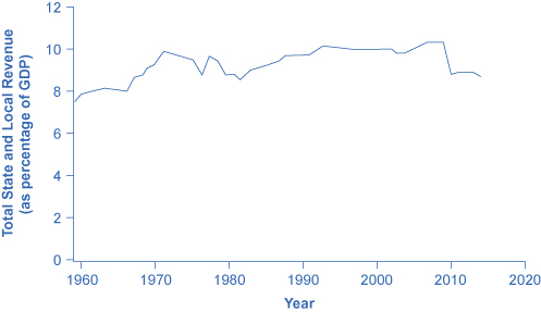
At the state and local level, taxes have been rising as a share of GDP over the last few decades to match the gradual rise in spending, as Figure 12.6 illustrates. The main revenue sources for state and local governments are sales taxes, property taxes, and revenue passed along from the federal government, but many state and local governments also levy personal and corporate income taxes, as well as impose a wide variety of fees and charges.
The specific sources of tax revenue vary widely across state and local governments. Some states rely more on property taxes, some on sales taxes, some on income taxes, and some more on revenues from the federal government.
The graph shows that total state and local revenue (as a percentage of GDP) was less than 8% in 1960. It has decreased a bit since 2013.
- The two main federal taxes are individual income taxes and payroll taxes that provide funds for Social Security and Medicare; these taxes together account for more than 80% of federal revenues.
- Other federal taxes include the corporate income tax, excise taxes on alcohol, gasoline and tobacco, and the estate and gift tax.
- A progressive tax is one, like the federal income tax, where those with higher incomes pay a higher share of taxes out of their income than those with lower incomes.
- A proportional tax is one, like the payroll tax for Medicare, where everyone pays the same share of taxes regardless of income level.
- A regressive tax is one, like the payroll tax (above a certain threshold) that supports Social Security, where those with high income pay a lower share of income in taxes than those with lower incomes.
- Suppose that gifts were taxed at a rate of 10% for amounts up to $100,000 and 20% for anything over that amount. Would this tax be regressive or progressive?
- If an individual owns a corporation for which he is the only employee, which different types of federal tax will he have to pay?
- What taxes would an individual pay if he were self-employed and the business is not incorporated?
- The social security tax is 6.2% on employees’ income earned below $113,000. Is this tax progressive, regressive or proportional?
- What are the main categories of U.S. federal government taxes?
- What is the difference between a progressive tax, a proportional tax, and a regressive tax?
- Excise taxes on tobacco and alcohol and state sales taxes are often criticized for being regressive. Although everyone pays the same rate regardless of income, why might this be so?
- What is the benefit of having state and local taxes on income instead of collecting all such taxes at the federal level?
12.3 Federal Deficits and the National Debt
Having discussed the revenue (taxes) and expense (spending) side of the budget, we now turn to the annual budget deficit or surplus, which is the difference between the tax revenue collected and spending over a fiscal year, which starts October 1 and ends September 30 of the next year.
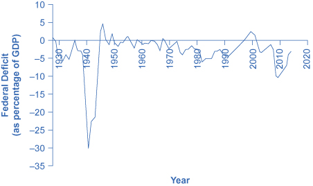
Figure 12.7 shows the pattern of annual federal budget deficits and surpluses, back to 1930, as a share of GDP. When the line is above the horizontal axis, the budget is in surplus. When the line is below the horizontal axis, a budget deficit occurred. Clearly, the biggest deficits as a share of GDP during this time were incurred to finance World War II. Deficits were also large during the 1930s, the 1980s, the early 1990s, and most recently during the 2008-2009 recession.
The graph shows that federal deficit (as a percentage of GDP) skyrocketed between the late 1930s and mid-1940s. In 2009, it was around –10%. In 2014, the federal deficit was close to –3%.
12.3.1 Debt/GDP Ratio
Another useful way to view the budget deficit is through the prism of accumulated debt rather than annual deficits. The national debt refers to the total amount that the government has borrowed over time. In contrast, the budget deficit refers to how much the government has borrowed in one particular year.
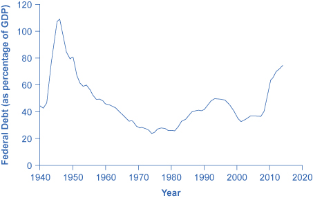
Figure 12.8 shows the ratio of debt/GDP since 1940. Until the 1970s, the debt/GDP ratio revealed a fairly clear pattern of federal borrowing. The government ran up large deficits and raised the debt/GDP ratio in World War II, but from the 1950s to the 1970s the government ran either surpluses or relatively small deficits, and so the debt/GDP ratio drifted down. Large deficits in the 1980s and early 1990s caused the ratio to rise sharply. When budget surpluses arrived from 1998 to 2001, the debt/GDP ratio declined substantially. The budget deficits starting in 2002 then tugged the debt/GDP ratio higher—with a big jump when the recession took hold in 2008–2009.
The graph shows that federal debt (as a percentage of GDP) was highest in the late 1940s before steadily declining down beneath 30% in the mid-1970s. Another increase took place during the recession in 2009 where it rose to over 60% and has been rising steadily since.
The next Clear it Up feature discusses how the government handles the national debt.
WHAT IS THE NATIONAL DEBT?
One year’s federal budget deficit causes the federal government to sell Treasury bonds to make up the difference between spending programs and tax revenues. The dollar value of all the outstanding Treasury bonds on which the federal government owes money is equal to the national debt.
12.3.2 The Path from Deficits to Surpluses to Deficits
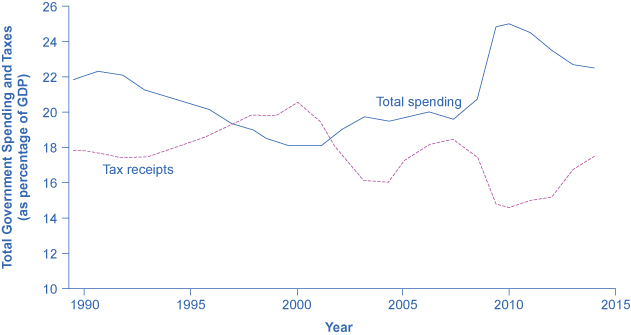
Why did the budget deficits suddenly turn to surpluses from 1998 to 2001 and why did the surpluses return to deficits in 2002? Why did the deficit become so large after 2007? Figure 12.9 suggests some answers. The graph combines the earlier information on total federal spending and taxes in a single graph, but focuses on the federal budget since 1990.
The graph shows that total spending and tax receipts rise and fall in contrast to one another. In 1990, total spending was around 22% whereas tax receipts which were just under 18%. In 2014, total spending was around 22% whereas tax receipts were around 17%.
Government spending as a share of GDP declined steadily through the 1990s. The biggest single reason was that defense spending declined from 5.2% of GDP in 1990 to 3.0% in 2000, but interest payments by the federal government also fell by about 1.0% of GDP. However, federal tax collections increased substantially in the later 1990s, jumping from 18.1% of GDP in 1994 to 20.8% in 2000. Powerful economic growth in the late 1990s fueled the boom in taxes. Personal income taxes rise as income goes up; payroll taxes rise as jobs and payrolls go up; corporate income taxes rise as profits go up. At the same time, government spending on transfer payments such as unemployment benefits, foods stamps, and welfare declined with more people working.
This sharp increase in tax revenues and decrease in expenditures on transfer payments was largely unexpected even by experienced budget analysts, and so budget surpluses came as a surprise. However, in the early 2000s, many of these factors started running in reverse. Tax revenues sagged, due largely to the recession that started in March 2001, which reduced revenues. Congress enacted a series of tax cuts and President George W. Bush signed them into law, starting in 2001. In addition, government spending swelled due to increases in defense, healthcare, education, Social Security, and support programs for those who were hurt by the recession and the slow growth that followed. Deficits returned. When the severe recession hit in late 2007, spending climbed and tax collections fell to historically unusual levels, resulting in enormous deficits.
Longer-term U.S. budget forecasts, a decade or more into the future, predict enormous deficits. The higher deficits during the 2008-2009 recession have repercussions, and the demographics will be challenging. The primary reason is the “baby boom”—the exceptionally high birthrates that began in 1946, right after World War II, and lasted for about two decades. Starting in 2010, the front edge of the baby boom generation began to reach age 65, and in the next two decades, the proportion of Americans over the age of 65 will increase substantially. The current level of the payroll taxes that support Social Security and Medicare will fall well short of the projected expenses of these programs, as the following Clear It Up feature shows; thus, the forecast is for large budget deficits. A decision to collect more revenue to support these programs or to decrease benefit levels would alter this long-term forecast.
WHAT IS THE LONG-TERM BUDGET OUTLOOK FOR SOCIAL SECURITY AND MEDICARE?
In 1946, just one American in 13 was over age 65. By 2000, it was one in eight. By 2030, one American in five will be over age 65. Two enormous U.S. federal programs focus on the elderly—Social Security and Medicare. The growing numbers of elderly Americans will increase spending on these programs, as well as on Medicaid. The current payroll tax levied on workers, which supports all of Social Security and the hospitalization insurance part of Medicare, will not be enough to cover the expected costs, so what are the options?
Long-term projections from the Congressional Budget Office in 2009 are that Medicare and Social Security spending combined will rise from 8.3% of GDP in 2009 to about 13% by 2035 and about 20% in 2080. If this rise in spending occurs, without any corresponding rise in tax collections, then some mix of changes must occur: (1) taxes will need to increase dramatically; (2) other spending will need to be cut dramatically; (3) the retirement age and/or age receiving Medicare benefits will need to increase, or (4) the federal government will need to run extremely large budget deficits.
Some proposals suggest removing the cap on wages subject to the payroll tax, so that those with very high incomes would have to pay the tax on the entire amount of their wages. Other proposals suggest moving Social Security and Medicare from systems in which workers pay for retirees toward programs that set up accounts where workers save funds over their lifetimes and then draw out after retirement to pay for healthcare.
The United States is not alone in this problem. Providing the promised level of retirement and health benefits to a growing proportion of elderly with a falling proportion of workers is an even more severe problem in many European nations and in Japan. How to pay promised levels of benefits to the elderly will be a difficult public policy decision.
In the next module we shift to the use of fiscal policy to counteract business cycle fluctuations. In addition, we will explore proposals requiring a balanced budget—that is, for government spending and taxes to be equal each year. The Impacts of Government Borrowing will also cover how fiscal policy and government borrowing will affect national saving—and thus affect economic growth and trade imbalances.
- For most of the twentieth century, the U.S. government took on debt during wartime and then paid down that debt slowly in peacetime.
- However, it took on quite substantial debts in peacetime in the 1980s and early 1990s, before a brief period of budget surpluses from 1998 to 2001, followed by a return to annual budget deficits since 2002, with very large deficits in the recession of 2008 and
- A budget deficit or budget surplus is measured annually.
- Total government debt or national debt is the sum of budget deficits and budget surpluses over time.
Debt has a certain self-reinforcing quality to it. There is one category of government spending that automatically increases along with the federal debt. What is it?
True or False:
 -   Federal spending has grown substantially in recent decades.
 -   By world standards, the U.S. government controls a
     relatively large share of the U.S. economy.
 -   A majority of the federal government's revenue is collected
     through personal income taxes.
 -   Education spending is slightly larger at the federal level
     than at the state and local level.
 -   State and local government spending has not risen much in
     recent decades.
 -   Defense spending is higher now than ever.
 -   The share of the economy going to federal taxes has
     increased substantially over time.
 -   Foreign aid is a large portion, although less than half, of
     federal spending.
 -   Federal deficits have been very large for the last two
     decades.
 -   The accumulated federal debt as a share of GDP is near an
     all-time high.
What has been the general pattern of U.S. budget deficits in recent decades?
What is the difference between a budget deficit and the national debt?
In a booming economy, is the federal government more likely to run surpluses or deficits? What are the various factors at play?
Economist Arthur Laffer famously pointed out that, in some cases, income tax revenue can actually go up when tax rates go down. Why might this be the case?
Is it possible for a nation to run budget deficits and still have its debt/GDP ratio fall? Explain your answer. Is it possible for a nation to run budget surpluses and still have its debt/GDP ratio rise? Explain your answer.
12.4 Using Fiscal Policy to Fight Recession, Unemployment, and Inflation
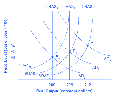
Fiscal policy is the use of government spending and tax policy to influence the path of the economy over time. Graphically, we see that fiscal policy, whether through changes in spending or taxes, shifts the aggregate demand outward in the case of expansionary fiscal policy and inward in the case of contractionary fiscal policy. We know from the chapter on economic growth that over time the quantity and quality of our resources grow as the population and thus the labor force get larger, as businesses invest in new capital, and as technology improves. The result of this is regular shifts to the right of the aggregate supply curves, as Figure 12.10 illustrates.
The original equilibrium occurs at E0, the intersection of aggregate demand curve AD0 and aggregate supply curve SRAS0, at an output level of 200 and a price level of 90. One year later, aggregate supply has shifted to the right to SRAS1 in the process of long-term economic growth, and aggregate demand has also shifted to the right to AD1, keeping the economy operating at the new level of potential GDP.
The new equilibrium (E1) is an output level of 206 and a price level of 92. One more year later, aggregate supply has again shifted to the right, now to SRAS2, and aggregate demand shifts right as well to AD2. Now the equilibrium is E2, with an output level of 212 and a price level of 94. In short, Figure 12.10 shows an economy that is growing steadily year to year, producing at its potential GDP each year, with only small inflationary increases in the price level.
Aggregate demand and aggregate supply do not always move neatly together. Think about what causes shifts in aggregate demand over time. As aggregate supply increases, incomes tend to go up. This tends to increase consumer and investment spending, shifting the aggregate demand curve to the right, but in any given period it may not shift the same amount as aggregate supply. What happens to government spending and taxes? Government spends to pay for the ordinary business of government- items such as national defense, social security, and healthcare, as Figure shows. Tax revenues, in part, pay for these expenditures. The result may be an increase in aggregate demand more than or less than the increase in aggregate supply. Aggregate demand may fail to increase along with aggregate supply, or aggregate demand may even shift left, for a number of possible reasons: households become hesitant about consuming; firms decide against investing as much; or perhaps the demand from other countries for exports diminishes.
For example, investment by private firms in physical capital in the U.S. economy boomed during the late 1990s, rising from 14.1% of GDP in 1993 to 17.2% in 2000, before falling back to 15.2% by 2002. Conversely, if shifts in aggregate demand run ahead of increases in aggregate supply, inflationary increases in the price level will result. Business cycles of recession and recovery are the consequence of shifts in aggregate supply and aggregate demand. As these occur, the government may choose to use fiscal policy to address the difference.
Monetary Policy and Bank Regulation shows us that a central bank can use its powers over the banking system to engage in countercyclical—or “against the business cycle”—actions. If recession threatens, the central bank uses an expansionary monetary policy to increase the money supply, increase the quantity of loans, reduce interest rates, and shift aggregate demand to the right. If inflation threatens, the central bank uses contractionary monetary policy to reduce the money supply, reduce the quantity of loans, raise interest rates, and shift aggregate demand to the left. Fiscal policy is another macroeconomic policy tool for adjusting aggregate demand by using either government spending or taxation policy.
12.4.1 Expansionary Fiscal Policy
Expansionary fiscal policy increases the level of aggregate demand, through either increases in government spending or reductions in tax rates. Expansionary policy can do this by (1) increasing consumption by raising disposable income through cuts in personal income taxes or payroll taxes; (2) increasing investment spending by raising after-tax profits through cuts in business taxes; and (3) increasing government purchases through increased federal government spending on final goods and services and raising federal grants to state and local governments to increase their expenditures on final goods and services. Contractionary fiscal policy does the reverse: it decreases the level of aggregate demand by decreasing consumption, decreasing investment, and decreasing government spending, either through cuts in government spending or increases in taxes. The aggregate demand/aggregate supply model is useful in judging whether expansionary or contractionary fiscal policy is appropriate.
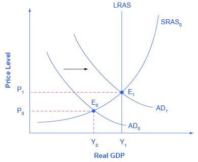
Consider first the situation in Figure 12.11, which is similar to the U.S. economy during the 2008-2009 recession. The intersection of aggregate demand (AD0) and aggregate supply (SRAS0) is occurring below the level of potential GDP as the LRAS curve indicates. At the equilibrium (E0), a recession occurs and unemployment rises. In this case, expansionary fiscal policy using tax cuts or increases in government spending can shift aggregate demand to AD1, closer to the full-employment level of output. In addition, the price level would rise back to the level P1 associated with potential GDP.
The graph shows two aggregate demand curves that each intersect with an aggregate supply curve. Aggregate demand curve (AD sub 1) intersects with both the aggregate supply curve (AS sub 0) as well as the potential GDP line.
Should the government use tax cuts or spending increases, or a mix of the two, to carry out expansionary fiscal policy? During the 2008-2009 Great Recession (which started, actually, in late 2007), the U.S. economy suffered a 3.1% cumulative loss of GDP. That may not sound like much, but it’s more than one year’s average growth rate of GDP. Over that time frame, the unemployment rate doubled from 5% to 10%. The consensus view is that this was possibly the worst economic downturn in U.S. history since the 1930’s Great Depression. The choice between whether to use tax or spending tools often has a political tinge. As a general statement, conservatives and Republicans prefer to see expansionary fiscal policy carried out by tax cuts, while liberals and Democrats prefer that the government implement expansionary fiscal policy through spending increases. In a bipartisan effort to address the extreme situation, the Obama administration and Congress passed an $830 billion expansionary policy in early 2009 involving both tax cuts and increases in government spending. At the same time, however, the federal stimulus was partially offset when state and local governments, whose budgets were hard hit by the recession, began cutting their spending.
The conflict over which policy tool to use can be frustrating to those who want to categorize economics as “liberal” or “conservative,” or who want to use economic models to argue against their political opponents. However, advocates of smaller government, who seek to reduce taxes and government spending can use the AD AS model, as well as advocates of bigger government, who seek to raise taxes and government spending. Economic studies of specific taxing and spending programs can help inform decisions about whether the government should change taxes or spending, and in what ways. Ultimately, decisions about whether to use tax or spending mechanisms to implement macroeconomic policy is a political decision rather than a purely economic one.
12.4.2 Contractionary Fiscal Policy
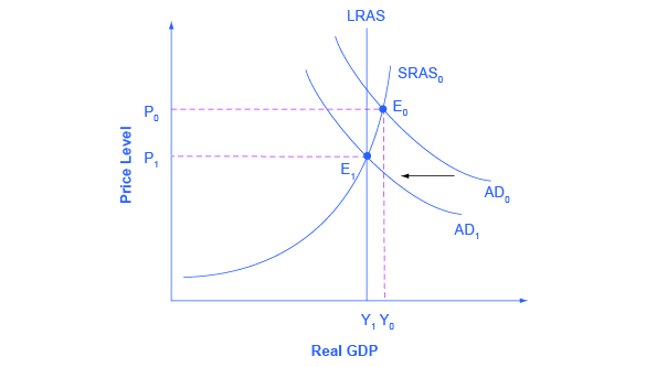
Fiscal policy can also contribute to pushing aggregate demand beyond potential GDP in a way that leads to inflation. As Figure 12.12 shows, a very large budget deficit pushes up aggregate demand, so that the intersection of aggregate demand (AD0) and aggregate supply (SRAS0) occurs at equilibrium E0, which is an output level above potential GDP. Economists sometimes call this an “overheating economy” where demand is so high that there is upward pressure on wages and prices, causing inflation. In this situation, contractionary fiscal policy involving federal spending cuts or tax increases can help to reduce the upward pressure on the price level by shifting aggregate demand to the left, to AD1, and causing the new equilibrium E1 to be at potential GDP, where aggregate demand intersects the LRAS curve.
The graph shows two aggregate demand curves that each intersect with an aggregate supply curve. Aggregate demand curve (AD sub 1) intersects with both the aggregate supply curve (AS sub 0) as well as the potential GDP line.
Again, the AD–AS model does not dictate how the government should carry out this contractionary fiscal policy. Some may prefer spending cuts; others may prefer tax increases; still others may say that it depends on the specific situation. The model only argues that, in this situation, the government needs to reduce aggregate demand.
- Expansionary fiscal policy increases the level of aggregate demand, either through increases in government spending or through reductions in taxes.
- Expansionary fiscal policy is most appropriate when an economy is in recession and producing below its potential GDP.
- Contractionary fiscal policy decreases the level of aggregate demand, either through cuts in government spending or increases in taxes.
- Contractionary fiscal policy is most appropriate when an economy is producing above its potential GDP.
- What is the main reason for employing contractionary fiscal policy in a time of strong economic growth?
- What is the main reason for employing expansionary fiscal policy during a recession?
- What is the difference between expansionary fiscal policy and contractionary fiscal policy?
- Under what general macroeconomic circumstances might a government use expansionary fiscal policy? When might it use contractionary fiscal policy?
- How will cuts in state budget spending affect federal expansionary policy?
- Is expansionary fiscal policy more attractive to politicians who believe in larger government or to politicians who believe in smaller government? Explain your answer.
12.5 Automatic Stabilizers
The millions of unemployed in 2008–2009 could collect unemployment insurance benefits to replace some of their salaries. Federal fiscal policies include discretionary fiscal policy, when the government passes a new law that explicitly changes tax or spending levels. The 2009 stimulus package is an example. Changes in tax and spending levels can also occur automatically, due to automatic stabilizers, such as unemployment insurance and food stamps, which are programs that are already laws that stimulate aggregate demand in a recession and hold down aggregate demand in a potentially inflationary boom.
12.5.1 Counterbalancing Recession and Boom
Consider first the situation where aggregate demand has risen sharply, causing the equilibrium to occur at a level of output above potential GDP. This situation will increase inflationary pressure in the economy. The policy prescription in this setting would be a dose of contractionary fiscal policy, implemented through some combination of higher taxes and lower spending. To some extent, both changes happen automatically. On the tax side, a rise in aggregate demand means that workers and firms throughout the economy earn more. Because taxes are based on personal income and corporate profits, a rise in aggregate demand automatically increases tax payments. On the spending side, stronger aggregate demand typically means lower unemployment and fewer layoffs, and so there is less need for government spending on unemployment benefits, welfare, Medicaid, and other programs in the social safety net.
The process works in reverse, too. If aggregate demand were to fall sharply so that a recession occurs, then the prescription would be for expansionary fiscal policy—some mix of tax cuts and spending increases. The lower level of aggregate demand and higher unemployment will tend to pull down personal incomes and corporate profits, an effect that will reduce the amount of taxes owed automatically. Higher unemployment and a weaker economy should lead to increased government spending on unemployment benefits, welfare, and other similar domestic programs. In 2009, the stimulus package included an extension in the time allowed to collect unemployment insurance. In addition, the automatic stabilizers react to a weakening of aggregate demand with expansionary fiscal policy and react to a strengthening of aggregate demand with contractionary fiscal policy, just as the AD/AS analysis suggests.
A combination of automatic stabilizers and discretionary fiscal policy produced the very large budget deficit in 2009. The Great Recession, starting in late 2007, meant less tax-generating economic activity, which triggered the automatic stabilizers that reduce taxes. Most economists, even those who are concerned about a possible pattern of persistently large budget deficits, are much less concerned or even quite supportive of larger budget deficits in the short run of a few years during and immediately after a severe recession.
A glance back at economic history provides a second illustration of the power of automatic stabilizers. Remember that the length of economic upswings between recessions has become longer in the U.S. economy in recent decades (as we discussed in Unemployment). The three longest economic booms of the twentieth century happened in the 1960s, the 1980s, and the 1991–2001 time period. One reason why the economy has tipped into recession less frequently in recent decades is that the size of government spending and taxes has increased in the second half of the twentieth century. Thus, the automatic stabilizing effects from spending and taxes are now larger than they were in the first half of the twentieth century. Around 1900, for example, federal spending was only about 2% of GDP. In 1929, just before the Great Depression hit, government spending was still just 4% of GDP. In those earlier times, the smaller size of government made automatic stabilizers far less powerful than in the last few decades, when government spending often hovers at 20% of GDP or more.
12.5.2 The Standardized Employment Deficit or Surplus
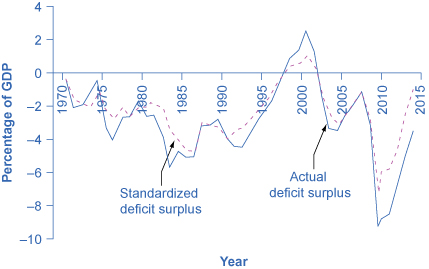
Each year, the nonpartisan Congressional Budget Office (CBO) calculates the standardized employment budget—that is, what the budget deficit or surplus would be if the economy were producing at potential GDP, where people who look for work were finding jobs in a reasonable period of time and businesses were making normal profits, with the result that both workers and businesses would be earning more and paying more taxes. In effect, the standardized employment deficit eliminates the impact of the automatic stabilizers. Figure 12.13 compares the actual budget deficits of recent decades with the CBO’s standardized deficit.
The graph shows how the standardized deficit surplus and the actual deficit surplus have changed since 1970. Both lines tend to rise and fall at similar times. The only time both were positive numbers was between the mid-1990s and early 2000s. As of 2014, both standardized deficit surplus and actual deficit surplus had dropped to their lowest amount, both below –6%.
Notice that in recession years, like the early 1990s, 2001, or 2009, the standardized employment deficit is smaller than the actual deficit. During recessions, the automatic stabilizers tend to increase the budget deficit, so if the economy was instead at full employment, the deficit would be reduced. However, in the late 1990s the standardized employment budget surplus was lower than the actual budget surplus. The gap between the standardized budget deficit or surplus and the actual budget deficit or surplus shows the impact of the automatic stabilizers. More generally, the standardized budget figures allow you to see what the budget deficit would look like with the economy held constant—at its potential GDP level of output.
Automatic stabilizers occur quickly. Lower wages means that a lower amount of taxes is withheld from paychecks right away. Higher unemployment or poverty means that government spending in those areas rises as quickly as people apply for benefits. However, while the automatic stabilizers offset part of the shifts in aggregate demand, they do not offset all or even most of it. Historically, automatic stabilizers on the tax and spending side offset about 10% of any initial movement in the level of output. This offset may not seem enormous, but it is still useful. Automatic stabilizers, like shock absorbers in a car, can be useful if they reduce the impact of the worst bumps, even if they do not eliminate the bumps altogether.
- Fiscal policy is conducted both through discretionary fiscal policy, which occurs when the government enacts taxation or spending changes in response to economic events, or through automatic stabilizers, which are taxing and spending mechanisms that, by their design, shift in response to economic events without any further legislation.
- The standardized employment budget is the calculation of what the budget deficit or budget surplus would have been in a given year if the economy had been producing at its potential GDP in that year.
- Many economists and politicians criticize the use of fiscal policy for a variety of reasons, including concerns over time lags, the impact on interest rates, and the inherently political nature of fiscal policy.
- We cover the critique of fiscal policy in the next module.
- In a recession, does the actual budget surplus or deficit fall above or below the standardized employment budget?
- What is the main advantage of automatic stabilizers over discretionary fiscal policy?
- Explain how automatic stabilizers work, both on the taxation side and on the spending side, first in a situation where the economy is producing less than potential GDP and then in a situation where the economy is producing more than potential GDP.
- What is the difference between discretionary fiscal policy and automatic stabilizers?
- Why do automatic stabilizers function “automatically?”
- What is the standardized employment budget?
- Is Medicaid (federal government aid to low-income families and individuals) an automatic stabilizer?
12.6 Practical Problems with Discretionary Fiscal Policy
In the early 1960s, many leading economists believed that the problem of the business cycle, and the swings between cyclical unemployment and inflation, were a thing of the past. On the cover of its December 31, 1965, issue, Time magazine, then the premier news magazine in the United States, ran a picture of John Maynard Keynes, and the story inside identified Keynesian theories as “the prime influence on the world’s economies.” The article reported that policymakers have “used Keynesian principles not only to avoid the violent [business] cycles of prewar days but to produce phenomenal economic growth and to achieve remarkably stable prices.”
This happy consensus, however, did not last. The U.S. economy suffered one recession from December 1969 to November 1970, a deeper recession from November 1973 to March 1975, and then double-dip recessions from January to June 1980 and from July 1981 to November 1982. At various times, inflation and unemployment both soared. Clearly, the problems of macroeconomic policy had not been completely solved. As economists began to consider what had gone wrong, they identified a number of issues that make discretionary fiscal policy more difficult than it had seemed in the rosy optimism of the mid-1960s.
12.6.1 Fiscal Policy and Interest Rates
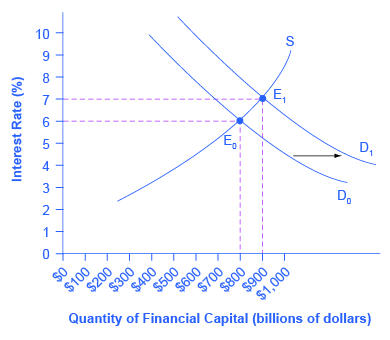
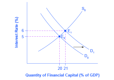
Because fiscal policy affects the quantity that the government borrows in financial capital markets, it not only affects aggregate demand—it can also affect interest rates. In Figure 12.14, the original equilibrium (E0) in the financial capital market occurs at a quantity of $800 billion and an interest rate of 6%. However, an increase in government budget deficits shifts the demand for financial capital from D0 to D1. The new equilibrium (E1) occurs at a quantity of $900 billion and an interest rate of 7%.
A consensus estimate based on a number of studies is that an increase in budget deficits (or a fall in budget surplus) by 1% of GDP will cause an increase of 0.5–1.0% in the long-term interest rate.
The graph shows two demand curves that each intersect with a supply curve. Demand curve (D sub 0) intersects with supply curve (S) at E sub 0 (point $800, 6%). Demand curve (D sub 1) intersects with supply curve (S) at E sub 1 (point $900, 7%).
A problem arises here. An expansionary fiscal policy, with tax cuts or spending increases, is intended to increase aggregate demand. If an expansionary fiscal policy also causes higher interest rates, then firms and households are discouraged from borrowing and spending (as occurs with tight monetary policy), thus reducing aggregate demand. Even if the direct effect of expansionary fiscal policy on increasing demand is not totally offset by lower aggregate demand from higher interest rates, fiscal policy can end up less powerful than was originally expected. We refer to this as crowding out, where government borrowing and spending results in higher interest rates, which reduces business investment and household consumption.
The broader lesson is that the government must coordinate fiscal and monetary policy. If expansionary fiscal policy is to work well, then the central bank can also reduce or keep short-term interest rates low. Conversely, monetary policy can also help to ensure that contractionary fiscal policy does not lead to a recession.
12.6.2 Long and Variable Time Lags
The government can change monetary policy several times each year, but it takes much longer to enact fiscal policy. Imagine that the economy starts to slow down. It often takes some months before the economic statistics signal clearly that a downturn has started, and a few months more to confirm that it is truly a recession and not just a one- or two-month blip. Economists often call the time it takes to determine that a recession has occurred the recognition lag. After this lag, policymakers become aware of the problem and propose fiscal policy bills. The bills go into various congressional committees for hearings, negotiations, votes, and then, if passed, eventually for the president’s signature.
- Inside Lag
-
Many fiscal policy bills about spending or taxes propose changes that would start in the next budget year or would be phased in gradually over time. Economists often refer to the time it takes to pass a bill as the legislative lag or inside lag.
- Outside Lag
-
Finally, once the government passes the bill it takes some time to disperse the funds to the appropriate agencies to implement the programs. Economists call the time it takes to start the projects the implementation lag or outside lag.
Moreover, the exact level of fiscal policy that the government should implement is never completely clear. Should it increase the budget deficit by 0.5% of GDP? By 1% of GDP? By 2% of GDP? In an AD/AS diagram, it is straightforward to sketch an aggregate demand curve shifting to the potential GDP level of output. In the real world, we only know roughly, not precisely, the actual level of potential output, and exactly how a spending cut or tax increase will affect aggregate demand is always somewhat controversial. Also unknown is the state of the economy at any point in time. During the early days of the Obama administration, for example, no one knew the true extent of the economy's deficit. During the 2008-2009 financial crisis, the rapid collapse of the banking system and automotive sector made it difficult to assess how quickly the economy was collapsing.
Thus, it can take many months or even more than a year to begin an expansionary fiscal policy after a recession has started—and even then, uncertainty will remain over exactly how much to expand or contract taxes and spending. When politicians attempt to use countercyclical fiscal policy to fight recession or inflation, they run the risk of responding to the macroeconomic situation of two or three years ago, in a way that may be exactly wrong for the economy at that time. George P. Schultz, a professor of economics, former Secretary of the Treasury, and Director of the Office of Management and Budget, once wrote: “While the economist is accustomed to the concept of lags, the politician likes instant results. The tension comes because, as I have seen on many occasions, the economist’s lag is the politician’s nightmare.”
12.6.3 Temporary and Permanent Fiscal Policy
A temporary tax cut or spending increase will explicitly last only for a year or two, and then revert to its original level. A permanent tax cut or spending increase is expected to stay in place for the foreseeable future. The effect of temporary and permanent fiscal policies on aggregate demand can be very different. Consider how you would react if the government announced a tax cut that would last one year and then be repealed, in comparison with how you would react if the government announced a permanent tax cut. Most people and firms will react more strongly to a permanent policy change than a temporary one.
This fact creates an unavoidable difficulty for countercyclical fiscal policy. The appropriate policy may be to have an expansionary fiscal policy with large budget deficits during a recession, and then a contractionary fiscal policy with budget surpluses when the economy is growing well. However, if both policies are explicitly temporary ones, they will have a less powerful effect than a permanent policy.
12.6.4 Structural Economic Change Takes Time
When an economy recovers from a recession, it does not usually revert to its exact earlier shape. Instead, the economy's internal structure evolves and changes and this process can take time. For example, much of the economic growth of the mid-2000s was in the construction sector (especially of housing) and finance. However, when housing prices started falling in 2007 and the resulting financial crunch led into recession (as we discussed in Monetary Policy and Bank Regulation), both sectors contracted. The manufacturing sector of the U.S. economy has been losing jobs in recent years as well, under pressure from technological change and foreign competition. Many of the people who lost work from these sectors in the 2008-2009 Great Recession will never return to the same jobs in the same sectors of the economy. Instead, the economy will need to grow in new and different directions, as the following Clear It Up feature shows. Fiscal policy can increase overall demand, but the process of structural economic change—the expansion of a new set of industries and the movement of workers to those industries—inevitably takes time.
WHY DO JOBS VANISH?
People can lose jobs for a variety of reasons: because of a recession, but also because of longer-run changes in the economy, such as new technology. Productivity improvements in auto manufacturing, for example, can reduce the number of workers needed, and eliminate these jobs in the long run. The internet has created jobs but also caused job loss, from travel agents to book store clerks. Many of these jobs may never come back. Short-run fiscal policy to reduce unemployment can create jobs, but it cannot replace jobs that will never return.
12.6.5 The Limitations of Fiscal Policy
Fiscal policy can help an economy that is producing below its potential GDP to expand aggregate demand so that it produces closer to potential GDP, thus lowering unemployment. However, fiscal policy cannot help an economy produce at an output level above potential GDP without causing inflation At this point, unemployment becomes so low that workers become scarce and wages rise rapidly.
12.6.6 Political Realties and Discretionary Fiscal Policy
A final problem for discretionary fiscal policy arises out of the difficulties of explaining to politicians how countercyclical fiscal policy that runs against the tide of the business cycle should work. Some politicians have a gut-level belief that when the economy and tax revenues slow down, it is time to hunker down, pinch pennies, and trim expenses. Countercyclical policy, however, says that when the economy has slowed, it is time for the government to stimulate the economy, raising spending, and cutting taxes. This offsets the drop in the economy in the other sectors. Conversely, when economic times are good and tax revenues are rolling in, politicians often feel that it is time for tax cuts and new spending. However, countercyclical policy says that this economic boom should be an appropriate time for keeping taxes high and restraining spending.
Politicians tend to prefer expansionary fiscal policy over contractionary policy. There is rarely a shortage of proposals for tax cuts and spending increases, especially during recessions. However, politicians are less willing to hear the message that in good economic times, they should propose tax increases and spending limits. In the economic upswing of the late 1990s and early 2000s, for example, the U.S. GDP grew rapidly. Estimates from respected government economic forecasters like the nonpartisan Congressional Budget Office and the Office of Management and Budget stated that the GDP was above potential GDP, and that unemployment rates were unsustainably low. However, no mainstream politician took the lead in saying that the booming economic times might be an appropriate time for spending cuts or tax increases. As of February 2017, President Trump has expressed plans to increase spending on national defense by 10% or $54 billion, increase infrastructure investment by $1 trillion, cut corporate and personal income taxes, all while maintaining the existing spending on Social Security and Medicare. The only way this math adds up is with a sizeable increase in the Federal budget deficit.
12.6.7 Discretionary Fiscal Policy: Summing Up
Expansionary fiscal policy can help to end recessions and contractionary fiscal policy can help to reduce inflation. Given the uncertainties over interest rate effects, time lags, temporary and permanent policies, and unpredictable political behavior, many economists and knowledgeable policymakers had concluded by the mid-1990s that discretionary fiscal policy was a blunt instrument, more like a club than a scalpel. It might still make sense to use it in extreme economic situations, like an especially deep or long recession. For less extreme situations, it was often preferable to let fiscal policy work through the automatic stabilizers and focus on monetary policy to steer short-term countercyclical efforts.
- Because fiscal policy affects the quantity of money that the government borrows in financial capital markets, it not only affects aggregate demand—it can also affect interest rates.
- If an expansionary fiscal policy also causes higher interest rates, then firms and households are discouraged from borrowing and spending, reducing aggregate demand in a situation called crowding out.
- Given the uncertainties over interest rate effects, time lags (implementation lag, legislative lag, and recognition lag), temporary and permanent policies, and unpredictable political behavior, many economists and knowledgeable policymakers have concluded that discretionary fiscal policy is a blunt instrument and better used only in extreme situations.
- What would happen if expansionary fiscal policy was implemented in a recession but, due to lag, did not actually take effect until after the economy was back to potential GDP?
- What would happen if contractionary fiscal policy were implemented during an economic boom but, due to lag, it did not take effect until the economy slipped into recession?
- Do you think the typical time lag for fiscal policy is likely to be longer or shorter than the time lag for monetary policy? Explain your answer?
- What are some practical weaknesses of discretionary fiscal policy?
- What is a potential problem with a temporary tax increase designed to increase aggregate demand if people know that it is temporary?
- If the government gives a $300 tax cut to everyone in the country, explain the mechanism by which this will cause interest rates to rise.
12.7 The Question of a Balanced Budget
For many decades, going back to the 1930s, various legislators have put forward proposals to require that the U.S. government balance its budget every year. In 1995, a proposed constitutional amendment that would require a balanced budget passed the U.S. House of Representatives by a wide margin, and failed in the U.S. Senate by only a single vote. (For the balanced budget to have become an amendment to the Constitution would have required a two-thirds vote by Congress and passage by three-quarters of the state legislatures.)
Most economists view the proposals for a perpetually balanced budget with bemusement. After all, in the short term, economists would expect the budget deficits and surpluses to fluctuate up and down with the economy and the automatic stabilizers. Economic recessions should automatically lead to larger budget deficits or smaller budget surpluses, while economic booms lead to smaller deficits or larger surpluses. A requirement that the budget be balanced each and every year would prevent these automatic stabilizers from working and would worsen the severity of economic fluctuations.
Some supporters of the balanced budget amendment like to argue that, since households must balance their own budgets, the government should too. However, this analogy between household and government behavior is severely flawed. Most households do not balance their budgets every year. Some years households borrow to buy houses or cars or to pay for medical expenses or college tuition. Other years they repay loans and save funds in retirement accounts. After retirement, they withdraw and spend those savings. Also, the government is not a household for many reasons, one of which is that the government has macroeconomic responsibilities. The argument of Keynesian macroeconomic policy is that the government needs to lean against the wind, spending when times are hard and saving when times are good, for the sake of the overall economy.
There is also no particular reason to expect a government budget to be balanced in the medium term of a few years. For example, a government may decide that by running large budget deficits, it can make crucial long-term investments in human capital and physical infrastructure that will build the country's long-term productivity. These decisions may work out well or poorly, but they are not always irrational. Such policies of ongoing government budget deficits may persist for decades. As the U.S. experience from the end of World War II up to about 1980 shows, it is perfectly possible to run budget deficits almost every year for decades, but as long as the percentage increases in debt are smaller than the percentage growth of GDP, the debt/GDP ratio will decline at the same time.
Nothing in this argument is a claim that budget deficits are always a wise policy. In the short run, a government that runs a very large budget deficit can shift aggregate demand to the right and trigger severe inflation. Additionally, governments may borrow for foolish or impractical reasons. The Impacts of Government Borrowing will discuss how large budget deficits, by reducing national saving, can in certain cases reduce economic growth and even contribute to international financial crises. A requirement that the budget be balanced in each calendar year, however, is a misguided overreaction to the fear that in some cases, budget deficits can become too large.
NO YELLOWSTONE PARK?
The 2013 federal budget shutdown illustrated the many sides to fiscal policy and the federal budget. In 2013, Republicans and Democrats could not agree on which spending policies to fund and how large the government debt should be. Due to the severity of the 2008-2009 recession, the fiscal stimulus, and previous policies, the federal budget deficit and debt was historically high. One way to try to cut federal spending and borrowing was to refuse to raise the legal federal debt limit, or tie on conditions to appropriation bills to stop the Affordable Health Care Act. This disagreement led to a two-week federal government shutdown and got close to the deadline where the federal government would default on its Treasury bonds. Finally, however, a compromise emerged and the government avoided default. This shows clearly how closely fiscal policies are tied to politics.
- Balanced budget amendments are a popular political idea, but the economic merits behind such proposals are questionable.
- Most economists accept that fiscal policy needs to be flexible enough to accommodate unforeseen expenditures, such as wars or recessions.
- While persistent, large budget deficits can indeed be a problem, a balanced budget amendment prevents even small, temporary deficits that might, in some cases, be necessary.
- How would a balanced budget amendment affect a decision by Congress to grant a tax cut during a recession?
- How would a balanced budget amendment change the effect of automatic stabilizer programs?
- What are some of the arguments for and against a requirement that the federal government budget be balanced every year?
- Do you agree or disagree with this statement: “It is in the best interest of our economy for Congress and the President to run a balanced budget each year.” Explain your answer.
- During the Great Recession of 2008–2009, what actions would have been required of Congress and the President had a balanced budget amendment to the Constitution been ratified? What impact would that have had on the unemployment rate?
12.8 Government Borrowing and Fiscal Debt
Governments have many competing demands for financial support. Any spending should be tempered by fiscal responsibility and by looking carefully at the spending’s impact. When a government spends more than it collects in taxes, it runs a budget deficit. It then needs to borrow. When government borrowing becomes especially large and sustained, it can substantially reduce the financial capital available to private sector firms, as well as lead to trade imbalances and even financial crises.
The Government Budgets and Fiscal Policy chapter introduced the concepts of deficits and debt, as well as how a government could use fiscal policy to address recession or inflation. This chapter begins by building on the national savings and investment identity, which we first first introduced in The International Trade and Capital Flows chapter, to show how government borrowing affects firms’ physical capital investment levels and trade balances. A prolonged period of budget deficits may lead to lower economic growth, in part because the funds that the government borrows to fund its budget deficits are typically no longer available for private investment. Moreover, a sustained pattern of large budget deficits can lead to disruptive economic patterns of high inflation, substantial inflows of financial capital from abroad, plummeting exchange rates, and heavy strains on a country’s banking and financial system.
FINANCING HIGHER EDUCATION
On November 8, 1965, President Lyndon B. Johnson signed The Higher Education Act of 1965 into law. With a stroke of the pen, he implemented what we know as the financial aid, work study, and student loan programs to help Americans pay for a college education. In his remarks, the President said:
Here the seeds were planted from which grew my firm conviction that for the individual, education is the path to achievement and fulfillment; for the Nation, it is a path to a society that is not only free but civilized; and for the world, it is the path to peace—for it is education that places reason over force.
This Act, he said, "is responsible for funding higher education for millions of Americans. It is the embodiment of the United States’ investment in ‘human capital’." Since Johnson signed the Act into law, the government has renewed it several times.
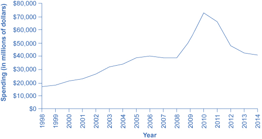
The purpose of The Higher Education Act of 1965 was to build the country’s human capital by creating educational opportunity for millions of Americans. The three criteria that the government uses to judge eligibility are income, full-time or part-time attendance, and the cost of the institution. According to the 2011–2012 National Postsecondary Student Aid Study (NPSAS:12), in the 2011–2012 school year, over 70% of all full-time college students received some form of federal financial aid; 47% received grants; and another 55% received federal government student loans. The budget to support financial aid has increased not only because of more enrollment, but also because of increased tuition and fees for higher education. The current Trump administration is currently questioning these increases and the entire notion of how the government should deal with higher education. The President and Congress are charged with balancing fiscal responsibility and important government-financed expenditures like investing in human capital.
12.9 How Government Borrowing Affects Investment and the Trade Balance
When governments are borrowers in financial markets, there are three possible sources for the funds from a macroeconomic point of view: (1) households might save more; (2) private firms might borrow less; and (3) the additional funds for government borrowing might come from outside the country, from foreign financial investors. Let’s begin with a review of why one of these three options must occur, and then explore how interest rates and exchange rates adjust to these connections.
12.9.1 The National Saving and Investment Identity
The national saving and investment identity, which we first introduced in The International Trade and Capital Flows chapter, provides a framework for showing the relationships between the sources of demand and supply in financial capital markets. The identity begins with a statement that must always hold true: the quantity of financial capital supplied in the market must equal the quantity of financial capital demanded.
The U.S. economy has two main sources for financial capital: private savings from inside the U.S. economy and public savings.
\[\text{Total savings} = \text{Private savings (S)} + \text{Public savings (T – G)}\]
These include the inflow of foreign financial capital from abroad. The inflow of savings from abroad is, by definition, equal to the trade deficit, as we explained in The International Trade and Capital Flows chapter. We can write this inflow of foreign investment capital as imports (M) minus exports (X). There are also two main sources of demand for financial capital: private sector investment (I) and government borrowing. Government borrowing in any given year is equal to the budget deficit, which we can write as the difference between government spending (G) and net taxes (T). Let’s call this equation 1.
\[\text{Quantity supplied of financial capital} = \text{Quantity demanded of financial capital}\]
\[\text{Private savings} + \text{Inflow of foreign savings} = \text{Private investment} + \text{Government budget deficit}\]
\[S + (M – X) = I + (G –T)\]
Governments often spend more than they receive in taxes and, therefore, public savings (T – G) is negative. This causes a need to borrow money in the amount of (G – T) instead of adding to the nation’s savings. If this is the case, we can view governments as demanders of financial capital instead of suppliers. In algebraic terms, we can rewrite the national savings and investment identity like this:
\[\text{Private investment} = \text{Private savings} + \text{Public savings} +\text{Trade deficit}\]
\[I = S + (T – G) + (M – X)\]
Let’s call this equation 2. We must accompany a change in any part of the national saving and investment identity by offsetting changes in at least one other part of the equation because we assume that the equality of quantity supplied and quantity demanded always holds. If the government budget deficit changes, then either private saving or investment or the trade balance—or some combination of the three—must change as well. Figure 12.16 shows the possible effects.
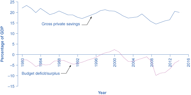
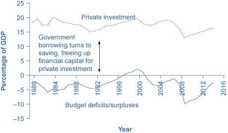
Following from the national savings and investment identity, charts (a) and (b) show what happens to investment, private savings, and the trade deficit when the budget deficit rises (or the budget surplus falls). (a) If the budget deficit rises (or the government budget surplus falls), the results could be (1) domestic private investment falls or (2) private savings rise or (3) the trade deficit increases (or a trade surplus diminishes). The opposite results of each are achieved when the budget deficit falls (or the budget surplus rises) as shown in image (b).
12.9.2 What about Budget Surpluses and Trade Surpluses?
The national saving and investment identity must always hold true because, by definition, the quantity supplied and quantity demanded in the financial capital market must always be equal. However, the formula will look somewhat different if the government budget is in deficit rather than surplus or if the balance of trade is in surplus rather than deficit. For example, in 1999 and 2000, the U.S. government had budget surpluses, although the economy was still experiencing trade deficits. When the government was running budget surpluses, it was acting as a saver rather than a borrower, and supplying rather than demanding financial capital. As a result, we would write the national saving and investment identity during this time as:
Quantity supplied of financial capital = Quantity demanded of financial capital
Private savings + Trade deficit + Government surplus = Private investment
\[S + (M – X) + (T – G)=I\]
Let's call this equation 3. Notice that this expression is mathematically the same as equation 2 except the savings and investment sides of the identity have simply flipped sides.
During the 1960s, the U.S. government was often running a budget deficit, but the economy was typically running trade surpluses. Since a trade surplus means that an economy is experiencing a net outflow of financial capital, we would write the national saving and investment identity as:
Quantity supplied of financial capital = Quantity demanded of financial capital
Private savings = Private investment + Outflow of foreign savings + Government budget deficit
Or using our math notation this reads:
\[S=I + (X – M) + (G – T)\]
Instead of the balance of trade representing part of the supply of financial capital, which occurs with a trade deficit, a trade surplus represents an outflow of financial capital leaving the domestic economy and invested elsewhere in the world.
Quantity supplied of financial capital = Quantity demanded of financial capital demand
Private savings = Private investment + Government budget deficit + Trade surplus
Using the math notation again, we have:
\[S=I + (G – T) + (X – M)\]
We assume that the point to these equations is that the national saving and investment identity always hold. When you write these relationships, it is important to engage your brain and think about what is on the supply and demand side of the financial capital market before you start your calculations.
As you can see in Figure 12.17, the Office of Management and Budget shows that the United States has consistently run budget deficits since 1977, with the exception of 1999 and 2000. What is alarming is the dramatic increase in budget deficits that has occurred since 2008, which in part reflects declining tax revenues and increased safety net expenditures due to the Great Recession. (Recall that T is net taxes. When the government must transfer funds back to individuals for safety net expenditures like Social Security and unemployment benefits, budget deficits rise.) These deficits have implications for the future health of the U.S. economy.
The graph shows U.S. government budgets and surpluses from 1977 to 2014. The United States has only had two years without a government budget deficit. In the 1980s the deficit hovered above –$200 million, gradually becoming a surplus by the end of 1990s. From 2000 onward, the deficit grew rapidly to –$600 million. The deficit was at its worst in 2009, at close to $1.6 trillion, following the Great Recession. In 2014, it was around –$514 million.
A rising budget deficit may result in a fall in domestic investment, a rise in private savings, or a rise in the trade deficit. The following modules discuss each of these possible effects in more detail.
- A change in any part of the national saving and investment identity suggests that if the government budget deficit changes, then either private savings, private investment in physical capital, or the trade balance—or some combination of the three—must change as well.
- In a country, private savings equals 600, the government budget surplus equals 200, and the trade surplus equals 100. What is the level of private investment in this economy?
- Assume an economy has a budget surplus of 1,000, private savings of 4,000, and investment of 5,000.
- Write out a national saving and investment identity for this economy.
- What will be the balance of trade in this economy?
- If the budget surplus changes to a budget deficit of 1000, with private saving and investment unchanged, what is the new balance of trade in this economy?
- Based on the national saving and investment identity, what are the three ways the macroeconomy might react to greater government budget deficits?
- How would you expect larger budget deficits to affect private sector investment in physical capital? Why?
- Assume there is no discretionary increase in government spending. Explain how an improving economy will affect the budget balance and, in turn, investment and the trade balance.
- Explain how decreased domestic investments that occur due to a budget deficit will affect future economic growth.
- The U.S. government has shut down a number of times in recent history. Explain how a government shutdown will affect the variables in the national investment and savings identity. Could the shutdown affect the government budget deficit?
12.10 Fiscal Policy and the Trade Balance
Government budget balances can affect the trade balance. As The Keynesian Perspective chapter discusses, a net inflow of foreign financial investment always accompanies a trade deficit, while a net outflow of financial investment always accompanies a trade surplus. One way to understand the connection from budget deficits to trade deficits is that when government creates a budget deficit with some combination of tax cuts or spending increases, it will increase aggregate demand in the economy, and some of that increase in aggregate demand will result in a higher level of imports. A higher level of imports, with exports remaining fixed, will cause a larger trade deficit. That means foreigners’ holdings of dollars increase as Americans purchase more imported goods. Foreigners use those dollars to invest in the United States, which leads to an inflow of foreign investment. One possible source of funding our budget deficit is foreigners buying Treasury securities that the U.S. government sells, thus a trade deficit often accompanies a budget deficit.
12.10.1 Twin Deficits?
In the mid-1980s, it was common to hear economists and even newspaper articles refer to the twin deficits, as the budget deficit and trade deficit both grew substantially. Figure 12.18 shows the pattern. The federal budget deficit went from 2.6% of GDP in 1981 to 5.1% of GDP in 1985—a drop of 2.5% of GDP. Over that time, the trade deficit moved from 0.5% in 1981 to 2.9% in 1985—a drop of 2.4% of GDP. In the mid-1980s an inflow of foreign investment capital matched, the considerable increase in government borrowing, so the government budget deficit and the trade deficit moved together.
The graph shows little relation between the rising (getting larger) and falling of the budget deficit and trade deficit since the 1980s.
Of course, no one should expect the budget deficit and trade deficit to move in lockstep, because the other parts of the national saving and investment identity—investment and private savings—will often change as well. In the late 1990s, for example, the government budget balance turned from deficit to surplus, but the trade deficit remained large and growing. During this time, the inflow of foreign financial investment was supporting a surge of physical capital investment by U.S. firms. In the first half of the 2000s, the budget and trade deficits again increased together, but in 2009, the budget deficit increased while the trade deficit declined. The budget deficit and the trade deficits are related to each other, but they are more like cousins than twins.
12.10.2 Budget Deficits and Exchange Rates
Exchange rates can also help to explain why budget deficits are linked to trade deficits. Figure 12.19 shows a situation using the exchange rate for the U.S. dollar, measured in euros. At the original equilibrium (E0), where the demand for U.S. dollars (D0) intersects with the supply of U.S. dollars (S0) on the foreign exchange market, the exchange rate is 0.9 euros per U.S. dollar and the equilibrium quantity traded in the market is $100 billion per day (which was roughly the quantity of dollar–euro trading in exchange rate markets in the mid-2000s). Then the U.S. budget deficit rises and foreign financial investment provides the source of funds for that budget deficit.
International financial investors, as a group, will demand more U.S. dollars on foreign exchange markets to purchase the U.S. government bonds, and they will supply fewer of the U.S. dollars that they already hold in these markets. Demand for U.S. dollars on the foreign exchange market shifts from D0 to D1 and the supply of U.S. dollars falls from S0 to S1. At the new equilibrium (E1), the exchange rate has appreciated to 1.05 euros per dollar while, in this example, the quantity of dollars traded remains the same.
This graph shows the demand and supply of foreign currency. The y-axis shows the euro/U.S. dollar exchange rate and the x-axis shows the quantity of dollars traded. As explained in the text, a budget deficit raises the demand for dollars (and lowers the supply of dollars) because foreign investors want to purchase U.S. government debt. The result is a stronger exchange rate.
A stronger exchange rate, of course, makes it more difficult for exporters to sell their goods abroad while making imports cheaper, so a trade deficit (or a reduced trade surplus) results. Thus, a budget deficit can easily result in an inflow of foreign financial capital, a stronger exchange rate, and a trade deficit.
You can also imagine interest rates are driving the exchange rate appreciation. As we explained earlier in [link], a budget deficit increases demand in markets for domestic financial capital, raising the domestic interest rate. A higher interest rate will attract an inflow of foreign financial capital, and appreciate the exchange rate in response to the increase in demand for U.S. dollars by foreign investors and a decrease in supply of U. S. dollars. Because of higher interest rates in the United States, Americans find U.S. bonds more attractive than foreign bonds. When Americans are buying fewer foreign bonds, they are supplying fewer U.S. dollars. U.S. dollar depreciation leads to a larger trade deficit (or reduced surplus). The connections between inflows of foreign investment capital, interest rates, and exchange rates are all just different ways of drawing the same economic connections: a larger budget deficit can result in a larger trade deficit, although do not expect the connection to be one-to-one.
12.10.3 From Budget Deficits to International Economic Crisis
We lay out step-by-step the economic story of how an outflow of international financial capital can cause a deep recession in the Exchange Rates and International Capital Flows chapter. When international financial investors decide to withdraw their funds from a country like Turkey, they increase the supply of the Turkish lira and reduce the demand for lira, depreciating the lira exchange rate. When firms and the government in a country like Turkey borrow money in international financial markets, they typically do so in stages. First, banks in Turkey borrow in a widely used currency like U.S. dollars or euros, then convert those U.S. dollars to lira, and then lend the money to borrowers in Turkey. If the lira's exchange rate value depreciates, then Turkey’s banks will find it impossible to repay the international loans that are in U.S. dollars or euros.
The combination of less foreign investment capital and banks that are bankrupt can sharply reduce aggregate demand, which causes a deep recession. Many countries around the world have experienced this kind of recession in recent years: along with Turkey in 2002, Mexico followed this general pattern in 1995, Thailand and countries across East Asia in 1997–1998, Russia in 1998, and Argentina in 2002. In many of these countries, large government budget deficits played a role in setting the stage for the financial crisis. A moderate increase in a budget deficit that leads to a moderate increase in a trade deficit and a moderate appreciation of the exchange rate is not necessarily a cause for concern. However, beyond some point that is hard to define in advance, a series of large budget deficits can become a cause for concern among international investors.
One reason for concern is that extremely large budget deficits mean that aggregate demand may shift so far to the right as to cause high inflation. The example of Turkey is a situation where very large budget deficits brought inflation rates well into double digits. In addition, very large budget deficits at some point begin to raise a fear that the government would not repay the borrowing. In the last 175 years, the government of Turkey has been unable to pay its debts and defaulted on its loans six times. Brazil’s government has been unable to pay its debts and defaulted on its loans seven times; Venezuela, nine times; and Argentina, five times. The risk of high inflation or a default on repaying international loans will worry international investors, since both factors imply that the rate of return on their investments in that country may end up lower than expected. If international investors start withdrawing the funds from a country rapidly, the scenario of less investment, a depreciated exchange rate, widespread bank failure, and deep recession can occur. The following Clear It Up feature explains other impacts of large deficits.
WHAT ARE THE RISKS OF CHRONIC LARGE DEFICITS IN THE UNITED STATES?
If a government runs large budget deficits for a sustained period of time, what can go wrong? According to a recent Brookings Institution report, a key risk of a large budget deficit is that government debt may grow too high compared to the country’s GDP growth. As debt grows, the national savings rate will decline, leaving less available in financial capital for private investment. The impact of chronically large budget deficits is as follows:
- As the population ages, there will be an increasing demand for government services that may cause higher government deficits. Government borrowing and its interest payments will pull resources away from domestic investment in human capital and physical capital that is essential to economic growth.
- Interest rates may start to rise so that the cost of financing government debt will rise as well, creating pressure on the government to reduce its budget deficits through spending cuts and tax increases. These steps will be politically painful, and they will also have a contractionary effect on aggregate demand in the economy.
- Rising percentage of debt to GDP will create uncertainty in the financial and global markets that might cause a country to resort to inflationary tactics to reduce the real value of the debt outstanding. This will decrease real wealth and damage confidence in the country’s ability to manage its spending. After all, if the government has borrowed at a fixed interest rate of, say, 5%, and it lets inflation rise above that 5%, then it will effectively be able to repay its debt at a negative real interest rate.
The conventional reasoning suggests that the relationship between sustained deficits that lead to high levels of government debt and long-term growth is negative. How significant this relationship is, how big an issue it is compared to other macroeconomic issues, and the direction of causality, is less clear.
What remains important to acknowledge is that the relationship between debt and growth is negative and that for some countries, the relationship may be stronger than in others. It is also important to acknowledge the direction of causality: does high debt cause slow growth, slow growth cause high debt, or are both high debt and slow growth the result of third factors? In our analysis, we have argued simply that high debt causes slow growth. There may be more to this debate than we have space to discuss here.
12.10.4 Using Fiscal Policy to Address Trade Imbalances
If a nation is experiencing the inflow of foreign investment capital associated with a trade deficit because foreign investors are making long-term direct investments in firms, there may be no substantial reason for concern. After all, many low-income nations around the world would welcome direct investment by multinational firms that ties them more closely into the global networks of production and distribution of goods and services. In this case, the inflows of foreign investment capital and the trade deficit are attracted by the opportunities for a good rate of return on private sector investment in an economy.
However, governments should beware of a sustained pattern of high budget deficits and high trade deficits. The danger arises in particular when the inflow of foreign investment capital is not funding long-term physical capital investment by firms, but instead is short-term portfolio investment in government bonds. When inflows of foreign financial investment reach high levels, foreign financial investors will be on the alert for any reason to fear that the country’s exchange rate may decline or the government may be unable to repay what it has borrowed on time. Just as a few falling rocks can trigger an avalanche; a relatively small piece of bad news about an economy can trigger an enormous outflow of short-term financial capital.
Reducing a nation’s budget deficit will not always be a successful method of reducing its trade deficit, because other elements of the national saving and investment identity, like private saving or investment, may change instead. In those cases when the budget deficit is the main cause of the trade deficit, governments should take steps to reduce their budget deficits, lest they make their economy vulnerable to a rapid outflow of international financial capital that could bring a deep recession.
FINANCING HIGHER EDUCATION
Between 1982 and 2012, the increases in the cost of a college education had far outpaced that of the income of the typical American family. According to President Obama’s research staff, the cost of education at a four-year public college increased by 257% compared to an increase in family incomes of only 16% over the prior 30 years. The ongoing debate over a balanced budget and proposed cutbacks accentuated the need to increase investment in human capital to grow the economy versus deepening the already significant debt levels of the U.S. government.
In summer 2013, President Obama presented a plan to make college more affordable that included increasing Pell Grant awards and the number of recipients, caps on interest rates for student loans, and providing education tax credits. In addition, the plan includes an accountability method for institutions of higher education that focuses on completion rates and creates a College Scorecard. Whether or not all these initiatives come to fruition remains to be seen, but they are indicative of creative approaches that government can take to meet its obligation from both a public and fiscal policy perspective.
- The government need not balance its budget every year.
- However, a sustained pattern of large budget deficits over time risks causing several negative macroeconomic outcomes: a shift to the right in aggregate demand that causes an inflationary increase in the price level; crowding out private investment in physical capital in a way that slows down economic growth; and creating a dependence on inflows of international portfolio investment which can sometimes turn into outflows of foreign financial investment that can be injurious to a macroeconomy.
- In the late 1990s, the U.S. government moved from a budget deficit to a budget surplus and the trade deficit in the U.S. economy grew substantially. Using the national saving and investment identity, what can you say about the direction in which saving and/or investment must have changed in this economy?
- Under what conditions will a larger budget deficit cause a trade deficit?
- Explain how a shift from a government budget deficit to a budget surplus might affect the exchange rate.
- Describe how a plan for reducing the government deficit might affect a college student, a young professional, and a middle-income family.
12.11 How Government Borrowing Affects Private Saving
A change in government budgets may impact private saving. Imagine that people watch government budgets and adjust their savings accordingly. For example, whenever the government runs a budget deficit, people might reason: “Well, a higher budget deficit means that I’m just going to owe more taxes in the future to pay off all that government borrowing, so I’ll start saving now.” If the government runs budget surpluses, people might reason: “With these budget surpluses (or lower budget deficits), interest rates are falling, so that saving is less attractive. Moreover, with a budget surplus the country will be able to afford a tax cut sometime in the future. I won’t bother saving as much now.”
The theory that rational private households might shift their saving to offset government saving or borrowing is known as Ricardian equivalence because the idea has intellectual roots in the writings of the early nineteenth-century economist David Ricardo (1772–1823). If Ricardian equivalence holds completely true, then in the national saving and investment identity, any change in budget deficits or budget surpluses would be completely offset by a corresponding change in private saving. As a result, changes in government borrowing would have no effect at all on either physical capital investment or trade balances.
In practice, the private sector only sometimes and partially adjusts its savings behavior to offset government budget deficits and surpluses. Figure 12.20 shows the patterns of U.S. government budget deficits and surpluses and the rate of private saving—which includes saving by both households and firms—since 1980. The connection between the two is not at all obvious.
In the mid-1980s, for example, government budget deficits were quite large, but there is no corresponding surge of private saving. However, when budget deficits turn to surpluses in the late 1990s, there is a simultaneous decline in private saving. When budget deficits get very large in 2008 and 2009, there is some sign of a rise in saving. A variety of statistical studies based on the U.S. experience suggests that when government borrowing increases by $1, private saving rises by about 30 cents. A World Bank study from the late 1990s, looking at government budgets and private saving behavior in countries around the world, found a similar result.
The graph shows that government borrowing and private investment sometimes rise and fall together. For example, between 1980 and 1984 the deficit as a percentage of GDP fell from –5 to –2% and the gross private savings as a percentage of GDP also fell from 22% to 20%. In 2014, the gross private savings as around 20%, and the budget deficit/surplus was closer to –3%.
Private saving does increase to some extent when governments run large budget deficits, and private saving falls when governments reduce deficits or run large budget surpluses. However, the offsetting effects of private saving compared to government borrowing are much less than one-to-one. In addition, this effect can vary a great deal from country to country, from time to time, and over the short and the long run.
If the funding for a larger budget deficit comes from international financial investors, then a trade deficit may accompany a budget deficit. In some countries, this pattern of twin deficits has set the stage for international financial investors first to send their funds to a country and cause an appreciation of its exchange rate and then to pull their funds out and cause a depreciation of the exchange rate and a financial crisis as well. It depends on whether funding comes from international financial investors.
- The theory of Ricardian equivalence holds that changes in private saving will offset changes in government borrowing or saving.
- Thus, greater private saving will offset higher budget deficits, while greater private borrowing will offset larger budget surpluses.
- If the theory holds true, then changes in government borrowing or saving would have no effect on private investment in physical capital or on the trade balance.
- However, empirical evidence suggests that the theory holds true only partially.
- Imagine an economy in which Ricardian equivalence holds. This economy has a budget deficit of 50, a trade deficit of 20, private savings of 130, and investment of 100. If the budget deficit rises to 70, how are the other terms in the national saving and investment identity affected?
- What is the theory of Ricardian equivalence?
- What does the concept of rationality have to do with Ricardian equivalence?
- Explain whether or not you agree with the premise of the Ricardian equivalence theory that rational people might reason: “Well, a higher budget deficit (surplus) means that I’m just going to owe more (less) taxes in the future to pay off all that government borrowing, so I’ll start saving (spending) now.” Why or why not?
12.12 Fiscal Policy, Investment, and Economic Growth
The underpinnings of economic growth are investments in physical capital, human capital, and technology, all set in an economic environment where firms and individuals can react to the incentives provided by well-functioning markets and flexible prices. Government borrowing can reduce the financial capital available for private firms to invest in physical capital. However, government spending can also encourage certain elements of long-term growth, such as spending on roads or water systems, on education, or on research and development that creates new technology.
12.12.1 Crowding Out Physical Capital Investment
A larger budget deficit will increase demand for financial capital. If private saving and the trade balance remain the same, then less financial capital will be available for private investment in physical capital. When government borrowing soaks up available financial capital and leaves less for private investment in physical capital, economists call the result crowding out.
To understand the potential impact of crowding out, consider the U.S. economy's situation before the exceptional circumstances of the recession that started in late 2007. In 2005, for example, the budget deficit was roughly 4% of GDP. Private investment by firms in the U.S. economy has hovered in the range of 14% to 18% of GDP in recent decades. However, in any given year, roughly half of U.S. investment in physical capital just replaces machinery and equipment that has worn out or become technologically obsolete. Only about half represents an increase in the total quantity of physical capital in the economy. Investment in new physical capital in any year is about 7% to 9% of GDP. In this situation, even U.S. budget deficits in the range of 4% of GDP can potentially crowd out a substantial share of new investment spending. Conversely, a smaller budget deficit (or an increased budget surplus) increases the pool of financial capital available for private investment.
Figure 12.21 shows the patterns of U.S. budget deficits and private investment since 1980. If greater government deficits lead to less private investment in physical capital, and reduced government deficits or budget surpluses lead to more investment in physical capital, these two lines should move up and down simultaneously. This pattern occurred in the late 1990s and early 2000s.
The U.S. federal budget went from a deficit of 2.2% of GDP in 1995 to a budget surplus of 2.4% of GDP in 2000—a swing of 4.6% of GDP. From 1995 to 2000, private investment in physical capital rose from 15% to 18% of GDP—a rise of 3% of GDP. Then, when the U.S. government again started running budget deficits in the early 2000s, less financial capital became available for private investment, and the rate of private investment fell back to about 15% of GDP by 2003.
The graph shows that in the case of the United States, since 1980 government borrowing and private investment have often risen and fallen in tandem. The y-axis shows U.S. government deficits/surpluses and private investment as a portion of GDP. The x-axis plots years from 1980 to 2014. It suggests that reduced government borrowing can free up capital for private investment.
This argument does not claim that a government's budget deficits will exactly shadow its national rate of private investment; after all, we must account for private saving and inflows of foreign financial investment. In the mid-1980s, for example, government budget deficits increased substantially without a corresponding drop off in private investment. In 2009, nonresidential private fixed investment dropped by $300 billion from its previous level of $1,941 billion in 2008, primarily because, during a recession, firms lack both the funds and the incentive to invest. Investment growth between 2009 and 2014 averaged approximately 5.9% to $2,210.5 billion—only slightly above its 2008 level, according to the Bureau of Economic Analysis. During that same period, interest rates dropped from 3.94% to less than a quarter percent as the Federal Reserve took dramatic action to prevent a depression by increasing the money supply through lowering short-term interest rates. The "crowding out" of private investment due to government borrowing to finance expenditures appears to have been suspended during the Great Recession. However, as the economy improves and interest rates rise, government borrowing may potentially create pressure on interest rates.
12.12.2 The Interest Rate Connection
Assume that government borrowing of substantial amounts will have an effect on the quantity of private investment. How will this affect interest rates in financial markets? In Figure 12.22, the original equilibrium (E0) where the demand curve (D0) for financial capital intersects with the supply curve (S0) occurs at an interest rate of 5% and an equilibrium quantity equal to 20% of GDP. However, as the government budget deficit increases, the demand curve for financial capital shifts from D0 to D1. The new equilibrium (E1) occurs at an interest rate of 6% and an equilibrium quantity of 21% of GDP.
The graph plots the downward-sloping demand and upward-sloping supply of financial capital. The y-axis is the interest rate (also known as the “price” of financial capital) and the x-axis shows the quantity of financial capital as a percentage of GDP. An increase in government borrowing increases the quantity of financial capital demanded at all interest rates. This is a rightward shift in the demand for financial capital. The graph shows that the equilibrium interest rate will rise.
A survey of economic studies on the connection between government borrowing and interest rates in the U.S. economy suggests that an increase of 1% in the budget deficit will lead to a rise in interest rates of between 0.5 and 1.0%, other factors held equal. In turn, a higher interest rate tends to discourage firms from making physical capital investments. One reason government budget deficits crowd out private investment, therefore, is the increase in interest rates. There are, however, economic studies that show a limited connection between the two (at least in the United States), but as the budget deficit grows, the dangers of rising interest rates become more real.
At this point, you may wonder about the Federal Reserve. After all, can the Federal Reserve not use expansionary monetary policy to reduce interest rates, or in this case, to prevent interest rates from rising? This useful question emphasizes the importance of considering how fiscal and monetary policies work in relation to each other. Imagine a central bank faced with a government that is running large budget deficits, causing a rise in interest rates and crowding out private investment. If the budget deficits are increasing aggregate demand when the economy is already producing near potential GDP, threatening an inflationary increase in price levels, the central bank may react with a contractionary monetary policy. In this situation, the higher interest rates from the government borrowing would be made even higher by contractionary monetary policy, and the government borrowing might crowd out a great deal of private investment.
Alternatively, if the budget deficits are increasing aggregate demand when the economy is producing substantially less than potential GDP, an inflationary increase in the price level is not much of a danger and the central bank might react with expansionary monetary policy. In this situation, higher interest rates from government borrowing would be largely offset by lower interest rates from expansionary monetary policy, and there would be little crowding out of private investment.
However, even a central bank cannot erase the overall message of the national savings and investment identity. If government borrowing rises, then private investment must fall, or private saving must rise, or the trade deficit must fall. By reacting with contractionary or expansionary monetary policy, the central bank can only help to determine which of these outcomes is likely.
12.12.3 Public Investment in Physical Capital
Government can invest in physical capital directly: roads and bridges; water supply and sewers; seaports and airports; schools and hospitals; plants that generate electricity, like hydroelectric dams or windmills; telecommunications facilities; and military weapons. In 2014, the U.S. federal government budget for Fiscal Year 2014 shows that the United States spent about $92 billion on transportation, including highways, mass transit, and airports.
Table 12.1 shows the federal government's total outlay for 2014 for major public physical capital investment in the United States. We have omitted physical capital related to the military or to residences where people live from this table, because the focus here is on public investments that have a direct effect on raising output in the private sector.
| Type of Public Physical Capital | Federal Outlays 2014 ($ millions) |
|---|---|
| Transportation | $91,915 |
| Community and regional development | $20,670 |
| Natural resources and the environment | $36,171 |
| Education, training, employment, and social services | $90,615 |
| Other | $37,282 |
| Total | $276,653 |
Public physical capital investment of this sort can increase the economy's output and productivity. An economy with reliable roads and electricity will be able to produce more. However, it is hard to quantify how much government investment in physical capital will benefit the economy, because government responds to political as well as economic incentives. When a firm makes an investment in physical capital, it is subject to the discipline of the market: If it does not receive a positive return on investment, the firm may lose money or even go out of business.
In some cases, lawmakers make investments in physical capital as a way of spending money in key politicians' districts. The result may be unnecessary roads or office buildings. Even if a project is useful and necessary, it might be done in a way that is excessively costly, because local contractors who make campaign contributions to politicians appreciate the extra business. Alternatively, governments sometimes do not make the investments they should because a decision to spend on infrastructure does not need to just make economic sense. It must be politically popular as well. Managing public investment cost-effectively can be difficult.
If a government decides to finance an investment in public physical capital with higher taxes or lower government spending in other areas, it need not worry that it is directly crowding out private investment. Indirectly however, higher household taxes could cut down on the level of private savings available and have a similar effect. If a government decides to finance an investment in public physical capital by borrowing, it may end up increasing the quantity of public physical capital at the cost of crowding out investment in private physical capital, which could be more beneficial to the economy.
12.12.4 Public Investment in Human Capital
In most countries, the government plays a large role in society's investment in human capital through the education system. A highly educated and skilled workforce contributes to a higher rate of economic growth. For the low-income nations of the world, additional investment in human capital seems likely to increase productivity and growth. For the United States, critics have raised tough questions about how much increases in government spending on education will improve the actual level of education.
Among economists, discussions of education reform often begin with some uncomfortable facts. As Figure 12.23 shows, spending per student for kindergarten through grade 12 (K–12) increased substantially in real dollars through 2010. The U.S. Census Bureau reports that current spending per pupil for elementary and secondary education rose from $5,001 in 1998 to $10,608 in 2012. However, as measured by standardized tests like the SAT, the level of student academic achievement has barely budged in recent decades. On international tests, U.S. students lag behind students from many other countries. (Of course, test scores are an imperfect measure of education for a variety of reasons. It would be difficult, however, to argue that there are not real problems in the U.S. education system and that the tests are just inaccurate.)
The line graph shows that government spending on education has continually increased from 1998 up until 2006, where it leveled off. In 2008, it increased dramatically from $35 to over $70 million. Since 2010, spending has steadily decreased to a little over $40 million in 2014.
The fact that increased financial resources have not brought greater measurable gains in student performance has led some education experts to question whether the problems may be due to structure, not just to the resources spent.
Other government programs seek to increase human capital either before or after the K–12 education system. Programs for early childhood education, like the federal Head Start program, are directed at families where the parents may have limited educational and financial resources. Government also offers substantial support for universities and colleges. For example, in the United States about 60% of students take at least a few college or university classes beyond the high school level. In Germany and Japan, about half of all students take classes beyond the comparable high school level. In the countries of Latin America, only about one student in four takes classes beyond the high school level, and in the nations of sub-Saharan Africa, only about one student in 20.
Not all spending on educational human capital needs to happen through the government: many college students in the United States pay a substantial share of the cost of their education. If low-income countries of the world are going to experience a widespread increase in their education levels for grade-school children, government spending seems likely to play a substantial role. For the U.S. economy, and for other high-income countries, the primary focus at this time is more on how to get a bigger return from existing spending on education and how to improve the performance of the average high school graduate, rather than dramatic increases in education spending.
12.12.5 How Fiscal Policy Can Improve Technology
Research and development (R&D) efforts are the lifeblood of new technology. According to the National Science Foundation, federal outlays for research, development, and physical plant improvements to various governmental agencies have remained at an average of 8.8% of GDP. About one-fifth of U.S. R&D spending goes to defense and space-oriented research. Although defense-oriented R&D spending may sometimes produce consumer-oriented spinoffs, R&D that is aimed at producing new weapons is less likely to benefit the civilian economy than direct civilian R&D spending.
Fiscal policy can encourage R&D using either direct spending or tax policy. Government could spend more on the R&D that it carries out in government laboratories, as well as expanding federal R&D grants to universities and colleges, nonprofit organizations, and the private sector. By 2014, the federal share of R&D outlays totaled $135.5 billion, or about 4% of the federal government's total budget outlays, according to data from the National Science Foundation. Fiscal policy can also support R&D through tax incentives, which allow firms to reduce their tax bill as they increase spending on research and development.
12.12.6 Summary of Fiscal Policy, Investment, and Economic Growth
Investment in physical capital, human capital, and new technology is essential for long-term economic growth, as Table 12.2 summarizes. In a market-oriented economy, private firms will undertake most of the investment in physical capital, and fiscal policy should seek to avoid a long series of outsized budget deficits that might crowd out such investment.
We will see the effects of many growth-oriented policies very gradually over time, as students are better educated, we make physical capital investments, and man invents and implements new technologies.
| Sector | Physical Capital | Human Capital | New Technology |
|---|---|---|---|
| Private Sector | New investment in property and equipment |
On-the-job training training |
Research and development development |
| Public Sector | Public infrastructure | Public education Job training |
Research and development encouraged through private sector incentives and direct spending. |
- Economic growth comes from a combination of investment in physical capital, human capital, and technology.
- Government borrowing can crowd out private sector investment in physical capital, but fiscal policy can also increase investment in publicly owned physical capital, human capital (education), and research and development.
- Possible methods for improving education and society’s investment in human capital include spending more money on teachers and other educational resources, and reorganizing the education system to provide greater incentives for success.
- Methods for increasing research and development spending to generate new technology include direct government spending on R&D and tax incentives for businesses to conduct additional R&D.
- Why have many education experts recently placed an emphasis on altering the incentives that U.S. schools face rather than on increasing their budgets? Without endorsing any of these proposals as especially good or bad, list some of the ways in which incentives for schools might be altered.
- What are some steps the government can take to encourage research and development?
- What are some of the ways fiscal policy might encourage economic growth?
- What are some fiscal policies for improving a society’s human capital?
- What are some fiscal policies for improving the technologies that the economy will have to draw upon in the future?
- Explain how cuts in funding for programs such as Head Start might affect the development of human capital in the United States.
- Explain why the government might prefer to provide incentives to private firms to do investment or research and development, rather than simply doing the spending itself?
- Under what condition would crowding out not inhibit long-run economic growth? Under what condition would crowding out impede long-run economic growth?
- What must take place for the government to run deficits without any crowding out?

