flowchart LR
  A[Hard edge] --> B(Round edge)
  B --> C{Decision}
  C --> D[Result one]
  C --> E[Result two]
Appendix B — Test Quarto Stuff
Also this here. And that here.
This is a book created from markdown and executable code.
B.1 Test Mermaid diagrams
B.2 Test Graphviz
We can also reference figures such as Figure fig-simple
B.3 Test Tables
See (JungTran2012JDE?) for additional discussion of literate programming.
| fruit | price |
|---|---|
| apple | 2.05 |
| pear | 1.37 |
| orange | 3.09 |
B.4 ## Air Quality with R code
We can use multiple languages like so.
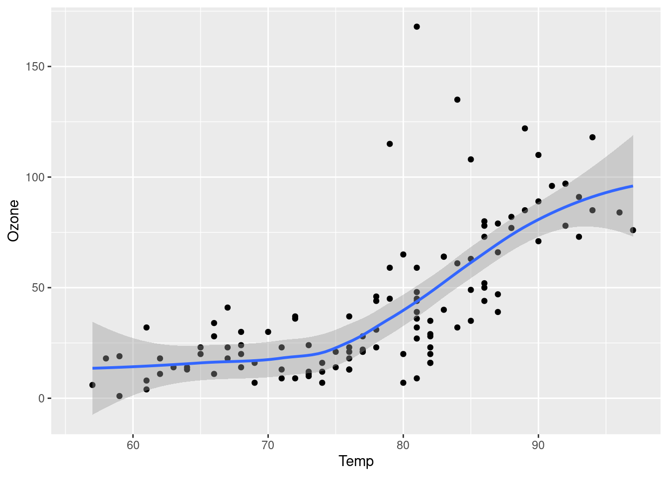
Figure fig-airquality further explores the impact of temperature on ozone level.
library(ggplot2)

ggplot(airquality, aes(Temp, Ozone)) +
  geom_point() +
  geom_smooth(method = "loess"
)
B.5 Python Code
1 + 12Markdown allows you to write using an easy-to-read, easy-to-write plain text format.
And then we add some more.
Note
Note that there are five types of callouts, including: note, tip, warning, caution, and important.
Tip With Caption
This is an example of a callout with a caption.
B.6 Math Stuff Code
We know from the first fundamental theorem of calculus that for \(x\) in \([a, b]\):
\[\frac{d}{dx}\left( \int_{a}^{x} f(u)\,du\right)=f(x).\]
For a demonstration of a line plot on a polar axis, see Figure fig-polar.
import numpy as np
import matplotlib.pyplot as plt

r = np.arange(0, 2, 0.01)
theta = 2 * np.pi * r
fig, ax = plt.subplots(
  subplot_kw = {'projection': 'polar'}
)

ax.plot(theta, r)
ax.set_rticks([0.5, 1, 1.5, 2])
ax.grid(True)
plt.show()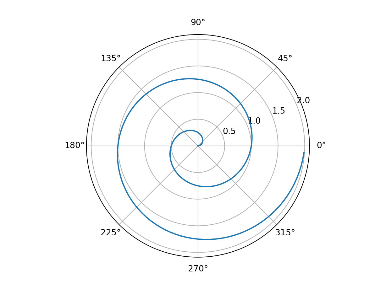
library(ggplot2)

ggplot(airquality, aes(Temp, Ozone)) +
  geom_point() +
  geom_smooth(method = "loess"
)
#| label: fig-parametric
#| fig-cap: "Parametric Plots"
using Plots
plot(sin,
     x->sin(2x),
     0,
     2π,
     leg=false,
     fill=(0,:lavender))
import numpy as np
import matplotlib.pyplot as plt
r = np.arange(0, 2, 0.01)
theta = 2 * np.pi * r
fig, ax = plt.subplots(
subplot_kw = {'projection': 'polar'}
)
ax.plot(theta, r)
ax.set_rticks([0.5, 1, 1.5, 2])
ax.grid(True)
plt.show()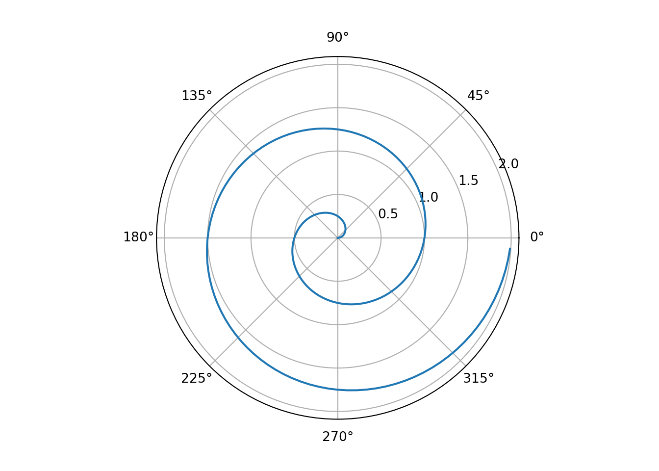
If this is really a new file then just do it.