import numpy as np
import pandas as pd
from matplotlib.pyplot import subplots
import statsmodels.api as sm
from ISLP import load_data
from ISLP.models import (ModelSpec as MS,
summarize)4 Lab Chapter 4: Logistic Regression, LDA, QDA, and KNN
4.1 The Stock Market Data
In this lab we will examine the Smarket data, which is part of the ISLP library. This data set consists of percentage returns for the S&P 500 stock index over 1,250 days, from the beginning of 2001 until the end of 2005. For each date, we have recorded the percentage returns for each of the five previous trading days, Lag1 through Lag5. We have also recorded Volume (the number of shares traded on the previous day, in billions), Today (the percentage return on the date in question) and Direction (whether the market was Up or Down on this date).
We start by importing our libraries at this top level; these are all imports we have seen in previous labs.
We also collect together the new imports needed for this lab.
from ISLP import confusion_table
from ISLP.models import contrast
from sklearn.discriminant_analysis import \
     (LinearDiscriminantAnalysis as LDA,
      QuadraticDiscriminantAnalysis as QDA)
from sklearn.naive_bayes import GaussianNB
from sklearn.neighbors import KNeighborsClassifier
from sklearn.preprocessing import StandardScaler
from sklearn.model_selection import train_test_split
from sklearn.linear_model import LogisticRegression
Now we are ready to load the Smarket data.
Smarket = load_data('Smarket')
Smarket| Year | Lag1 | Lag2 | Lag3 | Lag4 | Lag5 | Volume | Today | Direction | |
|---|---|---|---|---|---|---|---|---|---|
| 0 | 2001 | 0.381 | -0.192 | -2.624 | -1.055 | 5.010 | 1.19130 | 0.959 | Up |
| 1 | 2001 | 0.959 | 0.381 | -0.192 | -2.624 | -1.055 | 1.29650 | 1.032 | Up |
| 2 | 2001 | 1.032 | 0.959 | 0.381 | -0.192 | -2.624 | 1.41120 | -0.623 | Down |
| 3 | 2001 | -0.623 | 1.032 | 0.959 | 0.381 | -0.192 | 1.27600 | 0.614 | Up |
| 4 | 2001 | 0.614 | -0.623 | 1.032 | 0.959 | 0.381 | 1.20570 | 0.213 | Up |
| ... | ... | ... | ... | ... | ... | ... | ... | ... | ... |
| 1245 | 2005 | 0.422 | 0.252 | -0.024 | -0.584 | -0.285 | 1.88850 | 0.043 | Up |
| 1246 | 2005 | 0.043 | 0.422 | 0.252 | -0.024 | -0.584 | 1.28581 | -0.955 | Down |
| 1247 | 2005 | -0.955 | 0.043 | 0.422 | 0.252 | -0.024 | 1.54047 | 0.130 | Up |
| 1248 | 2005 | 0.130 | -0.955 | 0.043 | 0.422 | 0.252 | 1.42236 | -0.298 | Down |
| 1249 | 2005 | -0.298 | 0.130 | -0.955 | 0.043 | 0.422 | 1.38254 | -0.489 | Down |
1250 rows × 9 columns
This gives a truncated listing of the data. We can see what the variable names are.
Smarket.columnsIndex(['Year', 'Lag1', 'Lag2', 'Lag3', 'Lag4', 'Lag5', 'Volume', 'Today',
'Direction'],
dtype='object')We compute the correlation matrix using the corr() method for data frames, which produces a matrix that contains all of the pairwise correlations among the variables.
The pandas library does not report a correlation for the Direction variable because it is qualitative. This is why Smarket.corr() by itself would throw a value error that looks something like:
ValueError: could not convert string to float: 'Up'We therefore need to specify that correlations should only be calculated for numeric variables.
Smarket.corr(numeric_only=True)| Year | Lag1 | Lag2 | Lag3 | Lag4 | Lag5 | Volume | Today | |
|---|---|---|---|---|---|---|---|---|
| Year | 1.000000 | 0.029700 | 0.030596 | 0.033195 | 0.035689 | 0.029788 | 0.539006 | 0.030095 |
| Lag1 | 0.029700 | 1.000000 | -0.026294 | -0.010803 | -0.002986 | -0.005675 | 0.040910 | -0.026155 |
| Lag2 | 0.030596 | -0.026294 | 1.000000 | -0.025897 | -0.010854 | -0.003558 | -0.043383 | -0.010250 |
| Lag3 | 0.033195 | -0.010803 | -0.025897 | 1.000000 | -0.024051 | -0.018808 | -0.041824 | -0.002448 |
| Lag4 | 0.035689 | -0.002986 | -0.010854 | -0.024051 | 1.000000 | -0.027084 | -0.048414 | -0.006900 |
| Lag5 | 0.029788 | -0.005675 | -0.003558 | -0.018808 | -0.027084 | 1.000000 | -0.022002 | -0.034860 |
| Volume | 0.539006 | 0.040910 | -0.043383 | -0.041824 | -0.048414 | -0.022002 | 1.000000 | 0.014592 |
| Today | 0.030095 | -0.026155 | -0.010250 | -0.002448 | -0.006900 | -0.034860 | 0.014592 | 1.000000 |
As one would expect, the correlations between the lagged return variables and today’s return are close to zero. The only substantial correlation is between Year and Volume. By plotting the data we see that Volume is increasing over time. In other words, the average number of shares traded daily increased from 2001 to 2005.
Smarket.plot(y='Volume');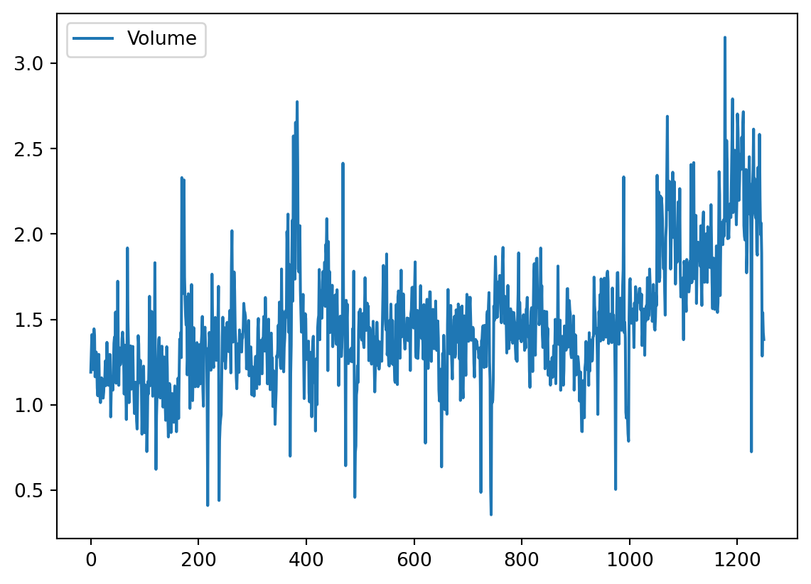
4.2 Logistic Regression
Next, we will fit a logistic regression model in order to predict Direction using Lag1 through Lag5 and Volume. The sm.GLM() function fits generalized linear models, a class of models that includes logistic regression. Alternatively, the function sm.Logit() fits a logistic regression model directly. The syntax of sm.GLM() is similar to that of sm.OLS(), except that we must pass in the argument family=sm.families.Binomial() in order to tell statsmodels to run a logistic regression rather than some other type of generalized linear model.
allvars = Smarket.columns.drop(['Today', 'Direction', 'Year'])
design = MS(allvars)
X = design.fit_transform(Smarket)
y = Smarket.Direction == 'Up'
glm = sm.GLM(y,
             X,
             family=sm.families.Binomial())
results = glm.fit()
summarize(results)| coef | std err | z | P>|z| | |
|---|---|---|---|---|
| intercept | -0.1260 | 0.241 | -0.523 | 0.601 |
| Lag1 | -0.0731 | 0.050 | -1.457 | 0.145 |
| Lag2 | -0.0423 | 0.050 | -0.845 | 0.398 |
| Lag3 | 0.0111 | 0.050 | 0.222 | 0.824 |
| Lag4 | 0.0094 | 0.050 | 0.187 | 0.851 |
| Lag5 | 0.0103 | 0.050 | 0.208 | 0.835 |
| Volume | 0.1354 | 0.158 | 0.855 | 0.392 |
The smallest p-value here is associated with Lag1. The negative coefficient for this predictor suggests that if the market had a positive return yesterday, then it is less likely to go up today. However, at a value of 0.15, the p-value is still relatively large, and so there is no clear evidence of a real association between Lag1 and Direction.
We use the params attribute of results in order to access just the coefficients for this fitted model.
results.paramsintercept -0.126000
Lag1 -0.073074
Lag2 -0.042301
Lag3 0.011085
Lag4 0.009359
Lag5 0.010313
Volume 0.135441
dtype: float64Likewise we can use the pvalues attribute to access the p-values for the coefficients.
results.pvaluesintercept 0.600700
Lag1 0.145232
Lag2 0.398352
Lag3 0.824334
Lag4 0.851445
Lag5 0.834998
Volume 0.392404
dtype: float64The predict() method of results can be used to predict the probability that the market will go up, given values of the predictors. This method returns predictions on the probability scale. If no data set is supplied to the predict() function, then the probabilities are computed for the training data that was used to fit the logistic regression model. As with linear regression, one can pass an optional exog argument consistent with a design matrix if desired. Here we have printed only the first ten probabilities.
probs = results.predict()
probs[:10]
array([0.50708413, 0.48146788, 0.48113883, 0.51522236, 0.51078116,
0.50695646, 0.49265087, 0.50922916, 0.51761353, 0.48883778])In order to make a prediction as to whether the market will go up or down on a particular day, we must convert these predicted probabilities into class labels, Up or Down. The following two commands create a vector of class predictions based on whether the predicted probability of a market increase is greater than or less than 0.5.
labels = np.array(['Down']*1250)
labels[probs>0.5] = "Up"
The confusion_table() function from the ISLP package summarizes these predictions, showing how many observations were correctly or incorrectly classified. Our function, which is adapted from a similar function in the module sklearn.metrics, transposes the resulting matrix and includes row and column labels. The confusion_table() function takes as first argument the predicted labels, and second argument the true labels.
confusion_table(labels, Smarket.Direction)| Truth | Down | Up |
|---|---|---|
| Predicted | ||
| Down | 145 | 141 |
| Up | 457 | 507 |
The diagonal elements of the confusion matrix indicate correct predictions, while the off-diagonals represent incorrect predictions. Hence our model correctly predicted that the market would go up on 507 days and that it would go down on 145 days, for a total of 507 + 145 = 652 correct predictions. The np.mean() function can be used to compute the fraction of days for which the prediction was correct. In this case, logistic regression correctly predicted the movement of the market 52.2% of the time.
(507+145)/1250, np.mean(labels == Smarket.Direction)(0.5216, 0.5216)At first glance, it appears that the logistic regression model is working a little better than random guessing. However, this result is misleading because we trained and tested the model on the same set of 1,250 observations. In other words, \(100-52.2=47.8%\) is the training error rate. As we have seen previously, the training error rate is often overly optimistic — it tends to underestimate the test error rate. In order to better assess the accuracy of the logistic regression model in this setting, we can fit the model using part of the data, and then examine how well it predicts the held out data. This will yield a more realistic error rate, in the sense that in practice we will be interested in our model’s performance not on the data that we used to fit the model, but rather on days in the future for which the market’s movements are unknown.
To implement this strategy, we first create a Boolean vector corresponding to the observations from 2001 through 2004. We then use this vector to create a held out data set of observations from 2005.
train = (Smarket.Year < 2005)
Smarket_train = Smarket.loc[train]
Smarket_test = Smarket.loc[~train]
Smarket_test.shape
(252, 9)The object train is a vector of 1,250 elements, corresponding to the observations in our data set. The elements of the vector that correspond to observations that occurred before 2005 are set to True, whereas those that correspond to observations in 2005 are set to False. Hence train is a boolean array, since its elements are True and False. Boolean arrays can be used to obtain a subset of the rows or columns of a data frame using the loc method. For instance, the command Smarket.loc[train] would pick out a submatrix of the stock market data set, corresponding only to the dates before 2005, since those are the ones for which the elements of train are True. The ~ symbol can be used to negate all of the elements of a Boolean vector. That is, ~train is a vector similar to train, except that the elements that are True in train get swapped to False in ~train, and vice versa. Therefore, Smarket.loc[~train] yields a subset of the rows of the data frame of the stock market data containing only the observations for which train is False. The output above indicates that there are 252 such observations.
We now fit a logistic regression model using only the subset of the observations that correspond to dates before 2005. We then obtain predicted probabilities of the stock market going up for each of the days in our test set — that is, for the days in 2005.
X_train, X_test = X.loc[train], X.loc[~train]
y_train, y_test = y.loc[train], y.loc[~train]
glm_train = sm.GLM(y_train,
                   X_train,
                   family=sm.families.Binomial())
results = glm_train.fit()
probs = results.predict(exog=X_test)
Notice that we have trained and tested our model on two completely separate data sets: training was performed using only the dates before 2005, and testing was performed using only the dates in 2005.
Finally, we compare the predictions for 2005 to the actual movements of the market over that time period. We will first store the test and training labels (recall y_test is binary).
D = Smarket.Direction
L_train, L_test = D.loc[train], D.loc[~train]
Now we threshold the fitted probability at 50% to form our predicted labels.
labels = np.array(['Down']*252)
labels[probs>0.5] = 'Up'
confusion_table(labels, L_test)| Truth | Down | Up |
|---|---|---|
| Predicted | ||
| Down | 77 | 97 |
| Up | 34 | 44 |
The test accuracy is about 48% while the error rate is about 52%
np.mean(labels == L_test), np.mean(labels != L_test)(0.4801587301587302, 0.5198412698412699)The != notation means not equal to, and so the last command computes the test set error rate. The results are rather disappointing: the test error rate is 52%, which is worse than random guessing! Of course this result is not all that surprising, given that one would not generally expect to be able to use previous days’ returns to predict future market performance. (After all, if it were possible to do so, then the authors of this book would be out striking it rich rather than writing a statistics textbook.)
We recall that the logistic regression model had very underwhelming p-values associated with all of the predictors, and that the smallest p-value, though not very small, corresponded to Lag1. Perhaps by removing the variables that appear not to be helpful in predicting Direction, we can obtain a more effective model. After all, using predictors that have no relationship with the response tends to cause a deterioration in the test error rate (since such predictors cause an increase in variance without a corresponding decrease in bias), and so removing such predictors may in turn yield an improvement. Below we refit the logistic regression using just Lag1 and Lag2, which seemed to have the highest predictive power in the original logistic regression model.
model = MS(['Lag1', 'Lag2']).fit(Smarket)
X = model.transform(Smarket)
X_train, X_test = X.loc[train], X.loc[~train]
glm_train = sm.GLM(y_train,
                   X_train,
                   family=sm.families.Binomial())
results = glm_train.fit()
probs = results.predict(exog=X_test)
labels = np.array(['Down']*252)
labels[probs>0.5] = 'Up'
confusion_table(labels, L_test)| Truth | Down | Up |
|---|---|---|
| Predicted | ||
| Down | 35 | 35 |
| Up | 76 | 106 |
Let’s evaluate the overall accuracy as well as the accuracy within the days when logistic regression predicts an increase.
(35+106)/252,106/(106+76)(0.5595238095238095, 0.5824175824175825)Now the results appear to be a little better: 56% of the daily movements have been correctly predicted. It is worth noting that in this case, a much simpler strategy of predicting that the market will increase every day will also be correct 56% of the time! Hence, in terms of overall error rate, the logistic regression method is no better than the naive approach. However, the confusion matrix shows that on days when logistic regression predicts an increase in the market, it has a 58% accuracy rate. This suggests a possible trading strategy of buying on days when the model predicts an increasing market, and avoiding trades on days when a decrease is predicted. Of course one would need to investigate more carefully whether this small improvement was real or just due to random chance.
Suppose that we want to predict the returns associated with particular values of Lag1 and Lag2. In particular, we want to predict Direction on a day when Lag1 and Lag2 equal \(1.2\) and \(1.1\), respectively, and on a day when they equal \(1.5\) and \(-0.8\). We do this using the predict() function.
newdata = pd.DataFrame({'Lag1':[1.2, 1.5],
                        'Lag2':[1.1, -0.8]});
newX = model.transform(newdata)
results.predict(newX)
0 0.479146
1 0.496094
dtype: float644.3 Linear Discriminant Analysis
We begin by performing LDA on the Smarket data, using the function LinearDiscriminantAnalysis(), which we have abbreviated LDA(). We fit the model using only the observations before 2005.
lda = LDA(store_covariance=True)Since the LDA estimator automatically adds an intercept, we should remove the column corresponding to the intercept in both X_train and X_test. We can also directly use the labels rather than the Boolean vectors y_train.
X_train, X_test = [M.drop(columns=['intercept'])
                   for M in [X_train, X_test]]
lda.fit(X_train, L_train)LinearDiscriminantAnalysis(store_covariance=True)In a Jupyter environment, please rerun this cell to show the HTML representation or trust the notebook.
On GitHub, the HTML representation is unable to render, please try loading this page with nbviewer.org.
LinearDiscriminantAnalysis(store_covariance=True)
Here we have used the list comprehensions introduced in Section 3.6.4. Looking at our first line above, we see that the right-hand side is a list of length two. This is because the code for M in [X_train, X_test] iterates over a list of length two. While here we loop over a list, the list comprehension method works when looping over any iterable object. We then apply the drop() method to each element in the iteration, collecting the result in a list. The left-hand side tells Python to unpack this list of length two, assigning its elements to the variables X_train and X_test. Of course, this overwrites the previous values of X_train and X_test.
Having fit the model, we can extract the means in the two classes with the means_ attribute. These are the average of each predictor within each class, and are used by LDA as estimates of \(\mu_k\). These suggest that there is a tendency for the previous 2 days’ returns to be negative on days when the market increases, and a tendency for the previous days’ returns to be positive on days when the market declines.
lda.means_array([[ 0.04279022, 0.03389409],
[-0.03954635, -0.03132544]])The estimated prior probabilities are stored in the priors_ attribute. The package sklearn typically uses this trailing _ to denote a quantity estimated when using the fit() method. We can be sure of which entry corresponds to which label by looking at the classes_ attribute.
lda.classes_array(['Down', 'Up'], dtype='<U4')The LDA output indicates that \(\hat\pi_{Down}=0.492\) and \(\hat\pi_{Up}=0.508\).
lda.priors_array([0.49198397, 0.50801603])The linear discriminant vectors can be found in the scalings_ attribute:
lda.scalings_array([[-0.64201904],
[-0.51352928]])These values provide the linear combination of Lag1 and Lag2 that are used to form the LDA decision rule. In other words, these are the multipliers of the elements of \(X=x\) in (4.24). If $-0.64Lag1 - 0.51 Lag2 $ is large, then the LDA classifier will predict a market increase, and if it is small, then the LDA classifier will predict a market decline.
lda_pred = lda.predict(X_test)As we observed in our comparison of classification methods (Section 4.5), the LDA and logistic regression predictions are almost identical.
confusion_table(lda_pred, L_test)| Truth | Down | Up |
|---|---|---|
| Predicted | ||
| Down | 35 | 35 |
| Up | 76 | 106 |
We can also estimate the probability of each class for each point in a training set. Applying a 50% threshold to the posterior probabilities of being in class 1 allows us to recreate the predictions contained in lda_pred.
lda_prob = lda.predict_proba(X_test)
np.all(
       np.where(lda_prob[:,1] >= 0.5, 'Up','Down') == lda_pred
)TrueAbove, we used the np.where() function that creates an array with value 'Up' for indices where the second column of lda_prob (the estimated posterior probability of 'Up') is greater than 0.5. For problems with more than two classes the labels are chosen as the class whose posterior probability is highest:
np.all(
       [lda.classes_[i] for i in np.argmax(lda_prob, 1)] == lda_pred
)TrueIf we wanted to use a posterior probability threshold other than 50% in order to make predictions, then we could easily do so. For instance, suppose that we wish to predict a market decrease only if we are very certain that the market will indeed decrease on that day — say, if the posterior probability is at least 90%. We know that the first column of lda_prob corresponds to the label Down after having checked the classes_ attribute, hence we use the column index 0 rather than 1 as we did above.
np.sum(lda_prob[:,0] > 0.9)0No days in 2005 meet that threshold! In fact, the greatest posterior probability of decrease in all of 2005 was 52.02%.
The LDA classifier above is the first classifier from the sklearn library. We will use several other objects from this library. The objects follow a common structure that simplifies tasks such as cross-validation, which we will see in Chapter 5. Specifically, the methods first create a generic classifier without referring to any data. This classifier is then fit to data with the fit() method and predictions are always produced with the predict() method. This pattern of first instantiating the classifier, followed by fitting it, and then producing predictions is an explicit design choice of sklearn. This uniformity makes it possible to cleanly copy the classifier so that it can be fit on different data; e.g. different training sets arising in cross-validation. This standard pattern also allows for a predictable formation of workflows.
4.4 Quadratic Discriminant Analysis
We will now fit a QDA model to the Smarket data. QDA is implemented via QuadraticDiscriminantAnalysis() in the sklearn package, which we abbreviate to QDA(). The syntax is very similar to LDA().
qda = QDA(store_covariance=True)
qda.fit(X_train, L_train)QuadraticDiscriminantAnalysis(store_covariance=True)In a Jupyter environment, please rerun this cell to show the HTML representation or trust the notebook.
On GitHub, the HTML representation is unable to render, please try loading this page with nbviewer.org.
QuadraticDiscriminantAnalysis(store_covariance=True)
The QDA() function will again compute means_ and priors_.
qda.means_, qda.priors_(array([[ 0.04279022, 0.03389409],
[-0.03954635, -0.03132544]]),
array([0.49198397, 0.50801603]))The QDA() classifier will estimate one covariance per class. Here is the estimated covariance in the first class:
qda.covariance_[0]array([[ 1.50662277, -0.03924806],
[-0.03924806, 1.53559498]])The output contains the group means. But it does not contain the coefficients of the linear discriminants, because the QDA classifier involves a quadratic, rather than a linear, function of the predictors. The predict() function works in exactly the same fashion as for LDA.
qda_pred = qda.predict(X_test)
confusion_table(qda_pred, L_test)| Truth | Down | Up |
|---|---|---|
| Predicted | ||
| Down | 30 | 20 |
| Up | 81 | 121 |
Interestingly, the QDA predictions are accurate almost 60% of the time, even though the 2005 data was not used to fit the model.
np.mean(qda_pred == L_test)0.5992063492063492This level of accuracy is quite impressive for stock market data, which is known to be quite hard to model accurately. This suggests that the quadratic form assumed by QDA may capture the true relationship more accurately than the linear forms assumed by LDA and logistic regression. However, we recommend evaluating this method’s performance on a larger test set before betting that this approach will consistently beat the market!
4.5 Naive Bayes
Next, we fit a naive Bayes model to the Smarket data. The syntax is similar to that of LDA() and QDA(). By default, this implementation GaussianNB() of the naive Bayes classifier models each quantitative feature using a Gaussian distribution. However, a kernel density method can also be used to estimate the distributions.
NB = GaussianNB()
NB.fit(X_train, L_train)GaussianNB()In a Jupyter environment, please rerun this cell to show the HTML representation or trust the notebook.
On GitHub, the HTML representation is unable to render, please try loading this page with nbviewer.org.
GaussianNB()
The classes are stored as classes_.
NB.classes_array(['Down', 'Up'], dtype='<U4')The class prior probabilities are stored in the class_prior_ attribute.
NB.class_prior_array([0.49198397, 0.50801603])The parameters of the features can be found in the theta_ and var_ attributes. The number of rows is equal to the number of classes, while the number of columns is equal to the number of features. We see below that the mean for feature Lag1 in the Down class is 0.043.
NB.theta_array([[ 0.04279022, 0.03389409],
[-0.03954635, -0.03132544]])Its variance is 1.503.
NB.var_array([[1.50355429, 1.53246749],
[1.51401364, 1.48732877]])How do we know the names of these attributes? We use NB? (or ?NB}).
We can easily verify the mean computation:
X_train[L_train == 'Down'].mean()Lag1 0.042790
Lag2 0.033894
dtype: float64Similarly for the variance:
X_train[L_train == 'Down'].var(ddof=0)Lag1 1.503554
Lag2 1.532467
dtype: float64Since NB() is a classifier in the sklearn library, making predictions uses the same syntax as for LDA() and QDA() above.
nb_labels = NB.predict(X_test)
confusion_table(nb_labels, L_test)| Truth | Down | Up |
|---|---|---|
| Predicted | ||
| Down | 29 | 20 |
| Up | 82 | 121 |
Naive Bayes performs well on these data, with accurate predictions over 59% of the time. This is slightly worse than QDA, but much better than LDA.
As for LDA, the predict_proba() method estimates the probability that each observation belongs to a particular class.
NB.predict_proba(X_test)[:5]array([[0.4873288 , 0.5126712 ],
[0.47623584, 0.52376416],
[0.46529531, 0.53470469],
[0.47484469, 0.52515531],
[0.49020587, 0.50979413]])4.6 K-Nearest Neighbors
We will now perform KNN using the KNeighborsClassifier() function. This function works similarly to the other model-fitting functions that we have encountered thus far.
As is the case for LDA and QDA, we fit the classifier using the fit method. New predictions are formed using the predict method of the object returned by fit().
knn1 = KNeighborsClassifier(n_neighbors=1)
knn1.fit(X_train, L_train)
knn1_pred = knn1.predict(X_test)
confusion_table(knn1_pred, L_test)| Truth | Down | Up |
|---|---|---|
| Predicted | ||
| Down | 43 | 58 |
| Up | 68 | 83 |
The results using \(K=1\) are not very good, since only \(50%\) of the observations are correctly predicted. Of course, it may be that \(K=1\) results in an overly-flexible fit to the data.
(83+43)/252, np.mean(knn1_pred == L_test)(0.5, 0.5)Below, we repeat the analysis using \(K=3\).
knn3 = KNeighborsClassifier(n_neighbors=3)
knn3_pred = knn3.fit(X_train, L_train).predict(X_test)
np.mean(knn3_pred == L_test)0.5317460317460317The results have improved slightly. But increasing K further provides no further improvements. It appears that for these data, and this train/test split, QDA gives the best results of the methods that we have examined so far.
KNN does not perform well on the Smarket data, but it often does provide impressive results. As an example we will apply the KNN approach to the Caravan data set, which is part of the ISLP library. This data set includes 85 predictors that measure demographic characteristics for 5,822 individuals. The response variable is Purchase, which indicates whether or not a given individual purchases a caravan insurance policy. In this data set, only 6% of people purchased caravan insurance.
Caravan = load_data('Caravan')
Purchase = Caravan.Purchase
Purchase.value_counts()
No 5474
Yes 348
Name: Purchase, dtype: int64The method value_counts() takes a pd.Series or pd.DataFrame and returns a pd.Series with the corresponding counts for each unique element. In this case Purchase has only Yes and No values and returns how many values of each there are.
348 / 58220.05977327378907592Our features will include all columns except Purchase.
feature_df = Caravan.drop(columns=['Purchase'])Because the KNN classifier predicts the class of a given test observation by identifying the observations that are nearest to it, the scale of the variables matters. Any variables that are on a large scale will have a much larger effect on the distance between the observations, and hence on the KNN classifier, than variables that are on a small scale. For instance, imagine a data set that contains two variables, salary and age (measured in dollars and years, respectively). As far as KNN is concerned, a difference of 1,000 USD in salary is enormous compared to a difference of 50 years in age. Consequently, salary will drive the KNN classification results, and age will have almost no effect. This is contrary to our intuition that a salary difference of 1,000 USD is quite small compared to an age difference of 50 years. Furthermore, the importance of scale to the KNN classifier leads to another issue: if we measured salary in Japanese yen, or if we measured age in minutes, then we’d get quite different classification results from what we get if these two variables are measured in dollars and years.
A good way to handle this problem is to standardize the data so that all variables are given a mean of zero and a standard deviation of one. Then all variables will be on a comparable scale. This is accomplished using the StandardScaler() transformation.
scaler = StandardScaler(with_mean=True,
                        with_std=True,
                        copy=True)
The argument with_mean indicates whether or not we should subtract the mean, while with_std indicates whether or not we should scale the columns to have standard deviation of 1 or not. Finally, the argument copy=True indicates that we will always copy data, rather than trying to do calculations in place where possible.
This transformation can be fit and then applied to arbitrary data. In the first line below, the parameters for the scaling are computed and stored in scaler, while the second line actually constructs the standardized set of features.
scaler.fit(feature_df)
X_std = scaler.transform(feature_df)
Now every column of feature_std below has a standard deviation of one and a mean of zero.
feature_std = pd.DataFrame(
                 X_std,
                 columns=feature_df.columns);
feature_std.std()
MOSTYPE 1.000086
MAANTHUI 1.000086
MGEMOMV 1.000086
MGEMLEEF 1.000086
MOSHOOFD 1.000086
...
AZEILPL 1.000086
APLEZIER 1.000086
AFIETS 1.000086
AINBOED 1.000086
ABYSTAND 1.000086
Length: 85, dtype: float64Notice that the standard deviations are not quite \(1\) here; this is again due to some procedures using the \(1/n\) convention for variances (in this case scaler()), while others use \(1/(n-1)\) (the std() method). See the footnote on page 198. In this case it does not matter, as long as the variables are all on the same scale.
Using the function train_test_split() we now split the observations into a test set, containing 1000 observations, and a training set containing the remaining observations. The argument random_state=0 ensures that we get the same split each time we rerun the code.
(X_train,
 X_test,
 y_train,
 y_test) = train_test_split(feature_std,
                            Purchase,
                            test_size=1000,
                            random_state=0)
?train_test_split reveals that the non-keyword arguments can be lists, arrays, pandas dataframes etc that all have the same length (shape[0]) and hence are indexable. In this case they are the dataframe feature_std and the response variable Purchase. We fit a KNN model on the training data using \(K=1\), and evaluate its performance on the test data.
knn1 = KNeighborsClassifier(n_neighbors=1)
knn1_pred = knn1.fit(X_train, y_train).predict(X_test)
np.mean(y_test != knn1_pred), np.mean(y_test != "No")
(0.111, 0.067)The KNN error rate on the 1,000 test observations is about \(11%\). At first glance, this may appear to be fairly good. However, since just over 6% of customers purchased insurance, we could get the error rate down to almost 6% by always predicting No regardless of the values of the predictors! This is known as the null rate.}
Suppose that there is some non-trivial cost to trying to sell insurance to a given individual. For instance, perhaps a salesperson must visit each potential customer. If the company tries to sell insurance to a random selection of customers, then the success rate will be only 6%, which may be far too low given the costs involved. Instead, the company would like to try to sell insurance only to customers who are likely to buy it. So the overall error rate is not of interest. Instead, the fraction of individuals that are correctly predicted to buy insurance is of interest.
confusion_table(knn1_pred, y_test)| Truth | No | Yes |
|---|---|---|
| Predicted | ||
| No | 880 | 58 |
| Yes | 53 | 9 |
It turns out that KNN with \(K=1\) does far better than random guessing among the customers that are predicted to buy insurance. Among 62 such customers, 9, or 14.5%, actually do purchase insurance. This is double the rate that one would obtain from random guessing.
9/(53+9)0.145161290322580664.6.1 Tuning Parameters
The number of neighbors in KNN is referred to as a tuning parameter, also referred to as a hyperparameter. We do not know a priori what value to use. It is therefore of interest to see how the classifier performs on test data as we vary these parameters. This can be achieved with a for loop, described in Section 2.3.8. Here we use a for loop to look at the accuracy of our classifier in the group predicted to purchase insurance as we vary the number of neighbors from 1 to 5:
for K in range(1,6):
    knn = KNeighborsClassifier(n_neighbors=K)
    knn_pred = knn.fit(X_train, y_train).predict(X_test)
    C = confusion_table(knn_pred, y_test)
    templ = ('K={0:d}: # predicted to rent: {1:>2},' +
            '  # who did rent {2:d}, accuracy {3:.1%}')
    pred = C.loc['Yes'].sum()
    did_rent = C.loc['Yes','Yes']
    print(templ.format(
          K,
          pred,
          did_rent,
          did_rent / pred))
K=1: # predicted to rent: 62, # who did rent 9, accuracy 14.5%
K=2: # predicted to rent: 6, # who did rent 1, accuracy 16.7%
K=3: # predicted to rent: 20, # who did rent 3, accuracy 15.0%
K=4: # predicted to rent: 4, # who did rent 0, accuracy 0.0%
K=5: # predicted to rent: 7, # who did rent 1, accuracy 14.3%We see some variability — the numbers for K=4 are very different from the rest.
4.6.2 Comparison to Logistic Regression
As a comparison, we can also fit a logistic regression model to the data. This can also be done with sklearn, though by default it fits something like the ridge regression version of logistic regression, which we introduce in Chapter 6. This can be modified by appropriately setting the argument C below. Its default value is 1 but by setting it to a very large number, the algorithm converges to the same solution as the usual (unregularized) logistic regression estimator discussed above.
Unlike the statsmodels package, sklearn focuses less on inference and more on classification. Hence, the summary methods seen in statsmodels and our simplified version seen with summarize are not generally available for the classifiers in sklearn.
logit = LogisticRegression(C=1e10, solver='liblinear')
logit.fit(X_train, y_train)
logit_pred = logit.predict_proba(X_test)
logit_labels = np.where(logit_pred[:,1] > 5, 'Yes', 'No')
confusion_table(logit_labels, y_test)| Truth | No | Yes |
|---|---|---|
| Predicted | ||
| No | 933 | 67 |
| Yes | 0 | 0 |
We used the argument solver='liblinear' above to avoid a warning with the default solver which would indicate that the algorithm does not converge.
If we use \(0.5\) as the predicted probability cut-off for the classifier, then we have a problem: none of the test observations are predicted to purchase insurance. However, we are not required to use a cut-off of \(0.5\). If we instead predict a purchase any time the predicted probability of purchase exceeds \(0.25\), we get much better results: we predict that 29 people will purchase insurance, and we are correct for about 31% of these people. This is almost five times better than random guessing!
logit_labels = np.where(logit_pred[:,1]>0.25, 'Yes', 'No')
confusion_table(logit_labels, y_test)| Truth | No | Yes |
|---|---|---|
| Predicted | ||
| No | 913 | 58 |
| Yes | 20 | 9 |
9/(20+9)0.31034482758620694.7 Linear and Poisson Regression on the Bikeshare Data
Here we fit linear and Poisson regression models to the Bikeshare data, as described in Section 4.6. The response bikers measures the number of bike rentals per hour in Washington, DC in the period 2010–2012.
Bike = load_data('Bikeshare')Let’s have a peek at the dimensions and names of the variables in this dataframe.
Bike.shape, Bike.columns((8645, 15),
Index(['season', 'mnth', 'day', 'hr', 'holiday', 'weekday', 'workingday',
'weathersit', 'temp', 'atemp', 'hum', 'windspeed', 'casual',
'registered', 'bikers'],
dtype='object'))4.7.1 Linear Regression
We begin by fitting a linear regression model to the data.
X = MS(['mnth',
        'hr',
        'workingday',
        'temp',
        'weathersit']).fit_transform(Bike)
Y = Bike['bikers']
M_lm = sm.OLS(Y, X).fit()
summarize(M_lm)| coef | std err | t | P>|t| | |
|---|---|---|---|---|
| intercept | -27.2068 | 6.715 | -4.052 | 0.000 |
| mnth[Aug] | 11.8181 | 4.698 | 2.515 | 0.012 |
| mnth[Dec] | 5.0328 | 4.280 | 1.176 | 0.240 |
| mnth[Feb] | -34.5797 | 4.575 | -7.558 | 0.000 |
| mnth[Jan] | -41.4249 | 4.972 | -8.331 | 0.000 |
| mnth[July] | 3.8996 | 5.003 | 0.779 | 0.436 |
| mnth[June] | 26.3938 | 4.642 | 5.686 | 0.000 |
| mnth[March] | -24.8735 | 4.277 | -5.815 | 0.000 |
| mnth[May] | 31.1322 | 4.150 | 7.501 | 0.000 |
| mnth[Nov] | 18.8851 | 4.099 | 4.607 | 0.000 |
| mnth[Oct] | 34.4093 | 4.006 | 8.589 | 0.000 |
| mnth[Sept] | 25.2534 | 4.293 | 5.883 | 0.000 |
| hr[1] | -14.5793 | 5.699 | -2.558 | 0.011 |
| hr[2] | -21.5791 | 5.733 | -3.764 | 0.000 |
| hr[3] | -31.1408 | 5.778 | -5.389 | 0.000 |
| hr[4] | -36.9075 | 5.802 | -6.361 | 0.000 |
| hr[5] | -24.1355 | 5.737 | -4.207 | 0.000 |
| hr[6] | 20.5997 | 5.704 | 3.612 | 0.000 |
| hr[7] | 120.0931 | 5.693 | 21.095 | 0.000 |
| hr[8] | 223.6619 | 5.690 | 39.310 | 0.000 |
| hr[9] | 120.5819 | 5.693 | 21.182 | 0.000 |
| hr[10] | 83.8013 | 5.705 | 14.689 | 0.000 |
| hr[11] | 105.4234 | 5.722 | 18.424 | 0.000 |
| hr[12] | 137.2837 | 5.740 | 23.916 | 0.000 |
| hr[13] | 136.0359 | 5.760 | 23.617 | 0.000 |
| hr[14] | 126.6361 | 5.776 | 21.923 | 0.000 |
| hr[15] | 132.0865 | 5.780 | 22.852 | 0.000 |
| hr[16] | 178.5206 | 5.772 | 30.927 | 0.000 |
| hr[17] | 296.2670 | 5.749 | 51.537 | 0.000 |
| hr[18] | 269.4409 | 5.736 | 46.976 | 0.000 |
| hr[19] | 186.2558 | 5.714 | 32.596 | 0.000 |
| hr[20] | 125.5492 | 5.704 | 22.012 | 0.000 |
| hr[21] | 87.5537 | 5.693 | 15.378 | 0.000 |
| hr[22] | 59.1226 | 5.689 | 10.392 | 0.000 |
| hr[23] | 26.8376 | 5.688 | 4.719 | 0.000 |
| workingday | 1.2696 | 1.784 | 0.711 | 0.477 |
| temp | 157.2094 | 10.261 | 15.321 | 0.000 |
| weathersit[cloudy/misty] | -12.8903 | 1.964 | -6.562 | 0.000 |
| weathersit[heavy rain/snow] | -109.7446 | 76.667 | -1.431 | 0.152 |
| weathersit[light rain/snow] | -66.4944 | 2.965 | -22.425 | 0.000 |
There are 24 levels in hr and 40 rows in all. In M_lm, the first levels hr[0] and mnth[Jan] are treated as the baseline values, and so no coefficient estimates are provided for them: implicitly, their coefficient estimates are zero, and all other levels are measured relative to these baselines. For example, the Feb coefficient of \(6.845\) signifies that, holding all other variables constant, there are on average about 7 more riders in February than in January. Similarly there are about 16.5 more riders in March than in January.
The results seen in Section 4.6.1 used a slightly different coding of the variables hr and mnth, as follows:
hr_encode = contrast('hr', 'sum')
mnth_encode = contrast('mnth', 'sum')
Refitting again:
X2 = MS([mnth_encode,
         hr_encode,
        'workingday',
        'temp',
        'weathersit']).fit_transform(Bike)
M2_lm = sm.OLS(Y, X2).fit()
S2 = summarize(M2_lm)
S2| coef | std err | t | P>|t| | |
|---|---|---|---|---|
| intercept | 73.5974 | 5.132 | 14.340 | 0.000 |
| mnth[Jan] | -46.0871 | 4.085 | -11.281 | 0.000 |
| mnth[Feb] | -39.2419 | 3.539 | -11.088 | 0.000 |
| mnth[March] | -29.5357 | 3.155 | -9.361 | 0.000 |
| mnth[April] | -4.6622 | 2.741 | -1.701 | 0.089 |
| mnth[May] | 26.4700 | 2.851 | 9.285 | 0.000 |
| mnth[June] | 21.7317 | 3.465 | 6.272 | 0.000 |
| mnth[July] | -0.7626 | 3.908 | -0.195 | 0.845 |
| mnth[Aug] | 7.1560 | 3.535 | 2.024 | 0.043 |
| mnth[Sept] | 20.5912 | 3.046 | 6.761 | 0.000 |
| mnth[Oct] | 29.7472 | 2.700 | 11.019 | 0.000 |
| mnth[Nov] | 14.2229 | 2.860 | 4.972 | 0.000 |
| hr[0] | -96.1420 | 3.955 | -24.307 | 0.000 |
| hr[1] | -110.7213 | 3.966 | -27.916 | 0.000 |
| hr[2] | -117.7212 | 4.016 | -29.310 | 0.000 |
| hr[3] | -127.2828 | 4.081 | -31.191 | 0.000 |
| hr[4] | -133.0495 | 4.117 | -32.319 | 0.000 |
| hr[5] | -120.2775 | 4.037 | -29.794 | 0.000 |
| hr[6] | -75.5424 | 3.992 | -18.925 | 0.000 |
| hr[7] | 23.9511 | 3.969 | 6.035 | 0.000 |
| hr[8] | 127.5199 | 3.950 | 32.284 | 0.000 |
| hr[9] | 24.4399 | 3.936 | 6.209 | 0.000 |
| hr[10] | -12.3407 | 3.936 | -3.135 | 0.002 |
| hr[11] | 9.2814 | 3.945 | 2.353 | 0.019 |
| hr[12] | 41.1417 | 3.957 | 10.397 | 0.000 |
| hr[13] | 39.8939 | 3.975 | 10.036 | 0.000 |
| hr[14] | 30.4940 | 3.991 | 7.641 | 0.000 |
| hr[15] | 35.9445 | 3.995 | 8.998 | 0.000 |
| hr[16] | 82.3786 | 3.988 | 20.655 | 0.000 |
| hr[17] | 200.1249 | 3.964 | 50.488 | 0.000 |
| hr[18] | 173.2989 | 3.956 | 43.806 | 0.000 |
| hr[19] | 90.1138 | 3.940 | 22.872 | 0.000 |
| hr[20] | 29.4071 | 3.936 | 7.471 | 0.000 |
| hr[21] | -8.5883 | 3.933 | -2.184 | 0.029 |
| hr[22] | -37.0194 | 3.934 | -9.409 | 0.000 |
| workingday | 1.2696 | 1.784 | 0.711 | 0.477 |
| temp | 157.2094 | 10.261 | 15.321 | 0.000 |
| weathersit[cloudy/misty] | -12.8903 | 1.964 | -6.562 | 0.000 |
| weathersit[heavy rain/snow] | -109.7446 | 76.667 | -1.431 | 0.152 |
| weathersit[light rain/snow] | -66.4944 | 2.965 | -22.425 | 0.000 |
What is the difference between the two codings? In M2_lm, a coefficient estimate is reported for all but level 23 of hr and level Dec of mnth. Importantly, in M2_lm, the (unreported) coefficient estimate for the last level of mnth is not zero: instead, it equals the negative of the sum of the coefficient estimates for all of the other levels. Similarly, in M2_lm, the coefficient estimate for the last level of hr is the negative of the sum of the coefficient estimates for all of the other levels. This means that the coefficients of hr and mnth in M2_lm will always sum to zero, and can be interpreted as the difference from the mean level. For example, the coefficient for January of \(-46.087\) indicates that, holding all other variables constant, there are typically 46 fewer riders in January relative to the yearly average.
It is important to realize that the choice of coding really does not matter, provided that we interpret the model output correctly in light of the coding used. For example, we see that the predictions from the linear model are the same regardless of coding:
np.sum((M_lm.fittedvalues - M2_lm.fittedvalues)**2)1.1303660379052135e-20The sum of squared differences is zero. We can also see this using the np.allclose() function:
np.allclose(M_lm.fittedvalues, M2_lm.fittedvalues)TrueTo reproduce the left-hand side of Figure 4.13 we must first obtain the coefficient estimates associated with mnth. The coefficients for January through November can be obtained directly from the M2_lm object. The coefficient for December must be explicitly computed as the negative sum of all the other months. We first extract all the coefficients for month from the coefficients of M2_lm.
coef_month = S2[S2.index.str.contains('mnth')]['coef']
coef_month
mnth[Jan] -46.0871
mnth[Feb] -39.2419
mnth[March] -29.5357
mnth[April] -4.6622
mnth[May] 26.4700
mnth[June] 21.7317
mnth[July] -0.7626
mnth[Aug] 7.1560
mnth[Sept] 20.5912
mnth[Oct] 29.7472
mnth[Nov] 14.2229
Name: coef, dtype: float64Next, we append Dec as the negative of the sum of all other months.
months = Bike['mnth'].dtype.categories
coef_month = pd.concat([
                       coef_month,
                       pd.Series([-coef_month.sum()],
                                  index=['mnth[Dec]'
                                 ])
                       ])
coef_month
mnth[Jan] -46.0871
mnth[Feb] -39.2419
mnth[March] -29.5357
mnth[April] -4.6622
mnth[May] 26.4700
mnth[June] 21.7317
mnth[July] -0.7626
mnth[Aug] 7.1560
mnth[Sept] 20.5912
mnth[Oct] 29.7472
mnth[Nov] 14.2229
mnth[Dec] 0.3705
dtype: float64Finally, to make the plot neater, we’ll just use the first letter of each month, which is the \(6\)th entry of each of the labels in the index.
fig_month, ax_month = subplots(figsize=(8,8))
x_month = np.arange(coef_month.shape[0])
ax_month.plot(x_month, coef_month, marker='o', ms=10)
ax_month.set_xticks(x_month)
ax_month.set_xticklabels([l[5] for l in coef_month.index], fontsize=20)
ax_month.set_xlabel('Month', fontsize=20)
ax_month.set_ylabel('Coefficient', fontsize=20);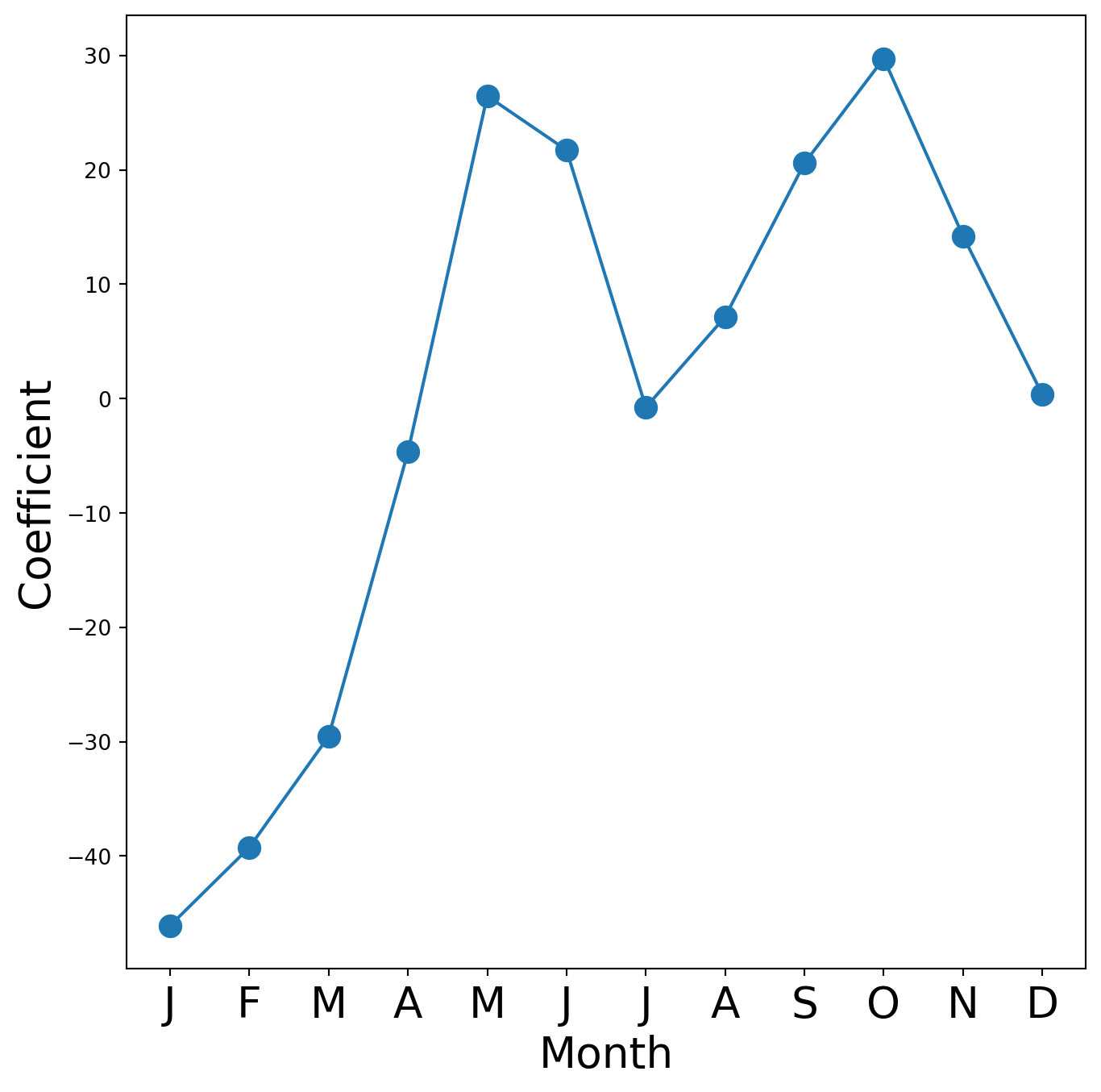
Reproducing the right-hand plot in Figure 4.13 follows a similar process.
coef_hr = S2[S2.index.str.contains('hr')]['coef']
coef_hr = coef_hr.reindex(['hr[{0}]'.format(h) for h in range(23)])
coef_hr = pd.concat([coef_hr,
                     pd.Series([-coef_hr.sum()], index=['hr[23]'])
                    ])
We now make the hour plot.
fig_hr, ax_hr = subplots(figsize=(8,8))
x_hr = np.arange(coef_hr.shape[0])
ax_hr.plot(x_hr, coef_hr, marker='o', ms=10)
ax_hr.set_xticks(x_hr[::2])
ax_hr.set_xticklabels(range(24)[::2], fontsize=20)
ax_hr.set_xlabel('Hour', fontsize=20)
ax_hr.set_ylabel('Coefficient', fontsize=20);
4.7.2 Poisson Regression
Now we fit instead a Poisson regression model to the Bikeshare data. Very little changes, except that we now use the function sm.GLM() with the Poisson family specified:
M_pois = sm.GLM(Y, X2, family=sm.families.Poisson()).fit()We can plot the coefficients associated with mnth and hr, in order to reproduce Figure 4.15. We first complete these coefficients as before.
S_pois = summarize(M_pois)
coef_month = S_pois[S_pois.index.str.contains('mnth')]['coef']
coef_month = pd.concat([coef_month,
                        pd.Series([-coef_month.sum()],
                                   index=['mnth[Dec]'])])
coef_hr = S_pois[S_pois.index.str.contains('hr')]['coef']
coef_hr = pd.concat([coef_hr,
                     pd.Series([-coef_hr.sum()],
                     index=['hr[23]'])])
The plotting is as before.
fig_pois, (ax_month, ax_hr) = subplots(1, 2, figsize=(16,8))
ax_month.plot(x_month, coef_month, marker='o', ms=10)
ax_month.set_xticks(x_month)
ax_month.set_xticklabels([l[5] for l in coef_month.index], fontsize=20)
ax_month.set_xlabel('Month', fontsize=20)
ax_month.set_ylabel('Coefficient', fontsize=20)
ax_hr.plot(x_hr, coef_hr, marker='o', ms=10)
ax_hr.set_xticklabels(range(24)[::2], fontsize=20)
ax_hr.set_xlabel('Hour', fontsize=20)
ax_hr.set_ylabel('Coefficient', fontsize=20);
/tmp/ipykernel_2792394/3779510511.py:8: UserWarning: FixedFormatter should only be used together with FixedLocator
ax_hr.set_xticklabels(range(24)[::2], fontsize=20)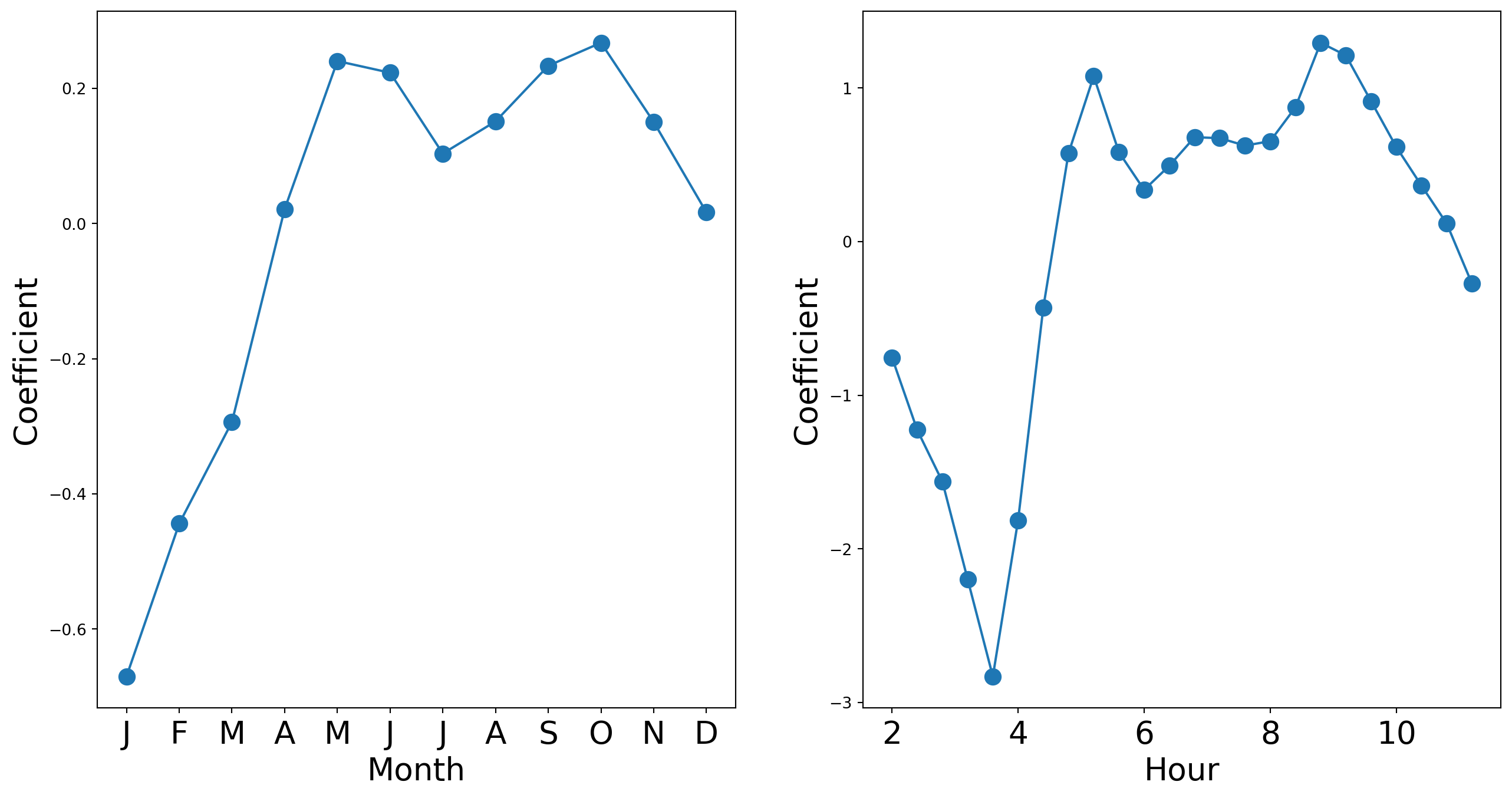
We compare the fitted values of the two models. The fitted values are stored in the fittedvalues attribute returned by the fit() method for both the linear regression and the Poisson fits. The linear predictors are stored as the attribute lin_pred.
fig, ax = subplots(figsize=(8, 8))
ax.scatter(M2_lm.fittedvalues,
           M_pois.fittedvalues,
           s=20)
ax.set_xlabel('Linear Regression Fit', fontsize=20)
ax.set_ylabel('Poisson Regression Fit', fontsize=20)
ax.axline([0,0], c='black', linewidth=3,
          linestyle='--', slope=1);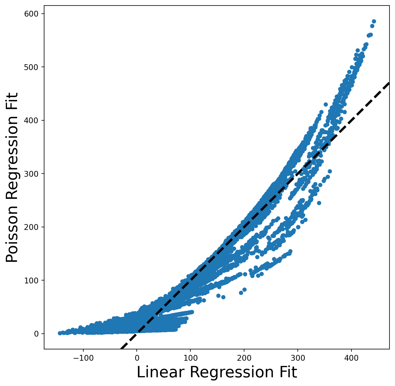
The predictions from the Poisson regression model are correlated with those from the linear model; however, the former are non-negative. As a result the Poisson regression predictions tend to be larger than those from the linear model for either very low or very high levels of ridership.
In this section, we fit Poisson regression models using the sm.GLM() function with the argument family=sm.families.Poisson(). Earlier in this lab we used the sm.GLM() function with family=sm.families.Binomial() to perform logistic regression. Other choices for the family argument can be used to fit other types of GLMs. For instance, family=sm.families.Gamma() fits a Gamma regression model.