20 Optimization

Chapter Learning Objectives

Univariate Function Optimization
Optimization Methods
Finding Root using Function Minimization
Multivariate Optimization

In this section I introduce algorithms that can find the minimum or maximum of a function. I will rely heavily on the previous chapter on root-finding. Many optimization problem can be recast as root-finding problems of the first derivative of the function that needs to be optimized.

As you have already noticed this book teaches by example. I will therefore first introduce the function that we will try "to optimize."

20.1 Univariate Function Optimization

import numpy as np
import matplotlib.pyplot as plt
import math as m
import time  # Imports system time module to time your script

plt.close('all')  # close all open figures

Here we want to optimize a univariate function:

$f (x) = 4 x^{2} e^{- 2 x}$

Think of it as a profit function of a company, where the argument of the function, the $x$ , is the amount of goods produced and subsequently sold. The more you produce and sell i.e., the larger the $x$ gets, the more profit you will make. But only up to a point. If you overdo it and start to produce too much, inefficiencies in production start to creep in possibly due to congestion in the production process or not enough demand so that production becomes wasteful and costlier the more you keep on producing. In other words, there is a sweet spot that you should not cross and if you do your profits will actually go down.

In Python we first define the function:

Python Code
R Code

def f_profit(x):
    if (x < 0):
        return (0)
    if (x == 0):
        return (np.nan)
    y = np.exp(-2*x)
    return (4 * x**2 * y)

f_profit <- function(x) {
  if (x < 0) {
    return (0)
  }
  if (x == 0) {
    return (NaN)
  }
  y <- exp(-2 * x)
  return (4 * x^2 * y)
}

# Test the R function with some values
result <- f_profit(2)
print(result)

[1] 0.2930502

Notice that I put a check into the function that returns zero for negative $x$ values. You cannot produce negative amounts, so we need to take care of this here.

Second I put a check in for zero value. Since you have a negative exponent, and x of zero would lead to a division by zero which usually breaks the code and returns a "division-by-zero" error. Mathematically a division by zero result in infinity. Infinity is not a problem for mathematical theory but it is a problem for numerical computation. We want to avoid it.

Plotting the function is always a good idea!

Python Code
R Code

xmin = 0.0
xmax = 6.0
xv = np.arange(xmin, xmax, (xmax - xmin)/200.0)
fx = np.zeros(len(xv),float) # define column vector
for i in range(len(xv)):
    fx[i] = f_profit(xv[i])

fig, ax = plt.subplots()
ax.plot(xv, fx)
ax.plot(xv, np.zeros(len(xv)))
ax.set_xlabel('x')
ax.set_ylabel('f(x)')
ax.set_title('Profit Function')
plt.show()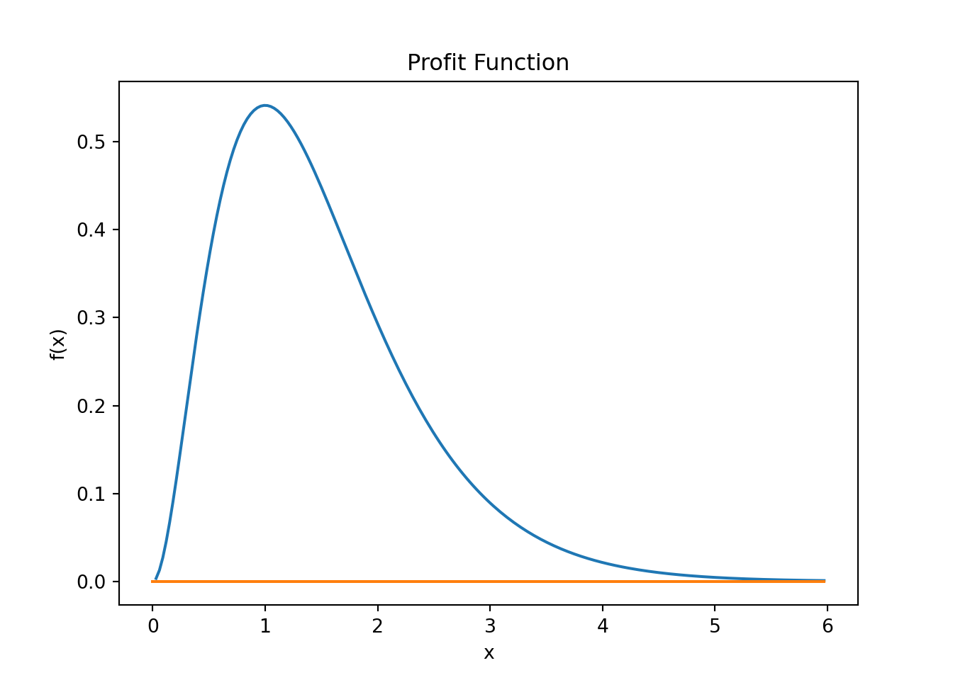

# Define the x values
xmin <- 0.0
xmax <- 6.0
xv <- seq(xmin, xmax, length.out = 200)

# Calculate the corresponding y values using the profit function
fx <- sapply(xv, f_profit)

# Create the plot
plot(xv, fx, type = "l", xlab = "x", ylab = "f(x)", main = "Profit Function")
abline(h = 0, col = "red")  # Add a horizontal line at y = 0 (red for emphasis)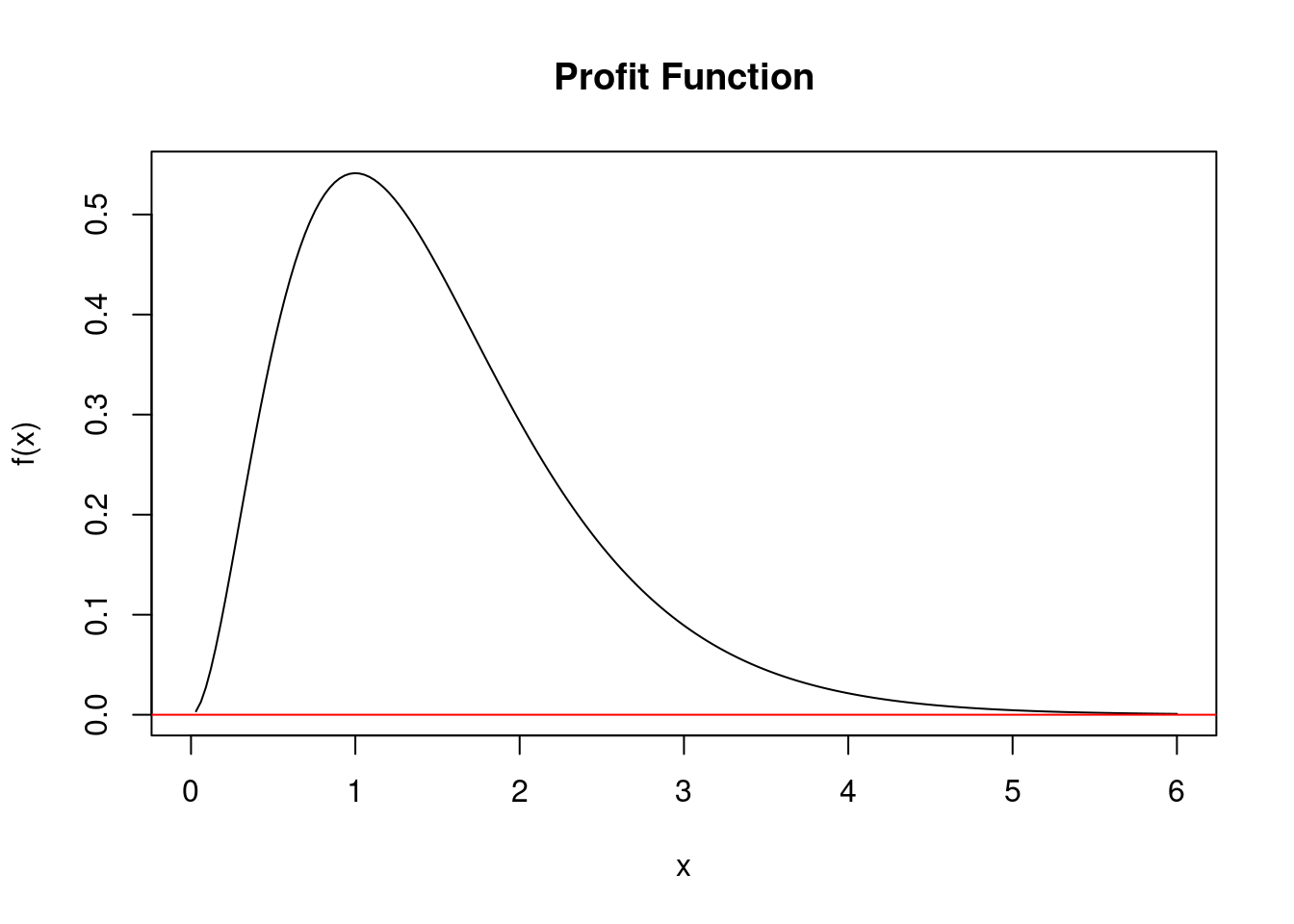

From the plot we see that this function seems to have a maximum around when $x \approx 1.0$ . It also seems to be the only maximum which would make it a global maximum.

20.2 Optimization Methods

20.2.1 Newton's Method

What do we know is true at the maximum? If you draw tangent lines along the function, we know that the tangent line at the maximum (or peak) of the function is a flat line. Like so:

Python Code
R Code

xmin = 0.0
xmax = 6.0
xv = np.linspace(xmin, xmax, 200)
fx = np.zeros(len(xv),float) # define column vector
for i in range(len(xv)):
    fx[i] = f_profit(xv[i])

fig, ax = plt.subplots()
ax.plot(xv, fx)
ax.plot(xv, f_profit(1)*np.ones(len(xv)))
ax.set_xlabel('x')
ax.set_ylabel('f(x)')
ax.set_title('Profit Function')
plt.show()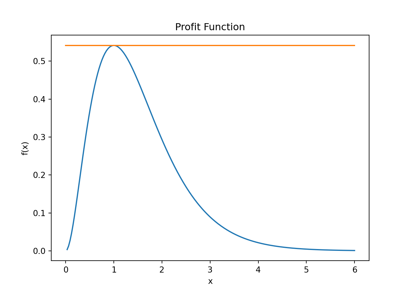

xmin <- 0.0
xmax <- 6.0
xv <- seq(xmin, xmax, length.out = 200)
fx <- rep(0, length(xv))

for (i in 1:length(xv)) {
  fx[i] <- f_profit(xv[i])
}

# Create the plot
plot(xv, fx, type = 'l', xlab = 'x', ylab = 'f(x)', main = 'Profit Function')
abline(h = f_profit(1), col = 'red')

Is there a mathematical expression for a tangent line? Yes there is, it is called the first derivative. This means that at the peak (i.e., maximum) of the function, the slope of the derivative is zero, right?

In other words, if we can find the $x$ value where the derivate of the function evaluates to zero, or $f^{'} (x) = 0$ , then we would have found the $x$ value where the function is at its maximum value.

Let's plot the derivative then and see where its value is zero. Calculus first. Derive the function and you will have:

$f^{'} (x) = 4 (2 \times x \times e^{- 2 x} + (- 2) x^{2} e^{- 2 x}) = 8 e^{- 2 x} x (1 - x)$

Derive it again (you will see shortly why) and you will get the second derivative:

$f^{″} (x) = 8 e^{- 2 x} (1 - 4 x + 2 x^{2})$

Next we define another Python function that returns all three, the function value $f (x)$ , the value of the derivative $f^{'} (x)$ , and the value of the second derivative $f^{″} (x)$ . Those are required by some of the algorithms that you are going to see shortly.

Python Code
R Code

def f_profit_plus_deriv(x):
    # gamma(2,3) density
    if (x < 0):
        return np.array([0, 0, 0])
    if (x == 0):
        return np.array([0, 0, np.nan])
    y = np.exp(-2.0*x)
    return np.array([4.0 * x**2.0 * np.exp(-2.0*x), \
      8.0 * np.exp(-2.0*x) * x*(1.0-x), \
      8.0 * np.exp(-2.0*x) * (1 - 4*x + 2 * x**2)])

f_profit_plus_deriv <- function(x) {
  if (x < 0) {
    return(c(0, 0, 0))
  }
  if (x == 0) {
    return(c(0, 0, NA))
  }
  y <- exp(-2 * x)
  return(c(4 * x^2 * exp(-2 * x), 8 * exp(-2 * x) * x * (1 - x), 8 * exp(-2 * x) * (1 - 4 * x + 2 * x^2)))
}

Python Code
R Code

xmin = 0.0
xmax = 6.0
xv = np.linspace(xmin, xmax, 200)
dfx = np.zeros(len(xv),float) # define column vector
for i in range(len(xv)):

    # The derivate value is in the second position
    dfx[i] = f_profit_plus_deriv(xv[i])[1]

fig, ax = plt.subplots()
ax.plot(xv, dfx)
ax.plot(xv, 0*np.ones(len(xv)))
ax.set_xlabel('x')
ax.set_ylabel('f\'(x)')
ax.set_title('Derivative of Profit Function')
plt.show()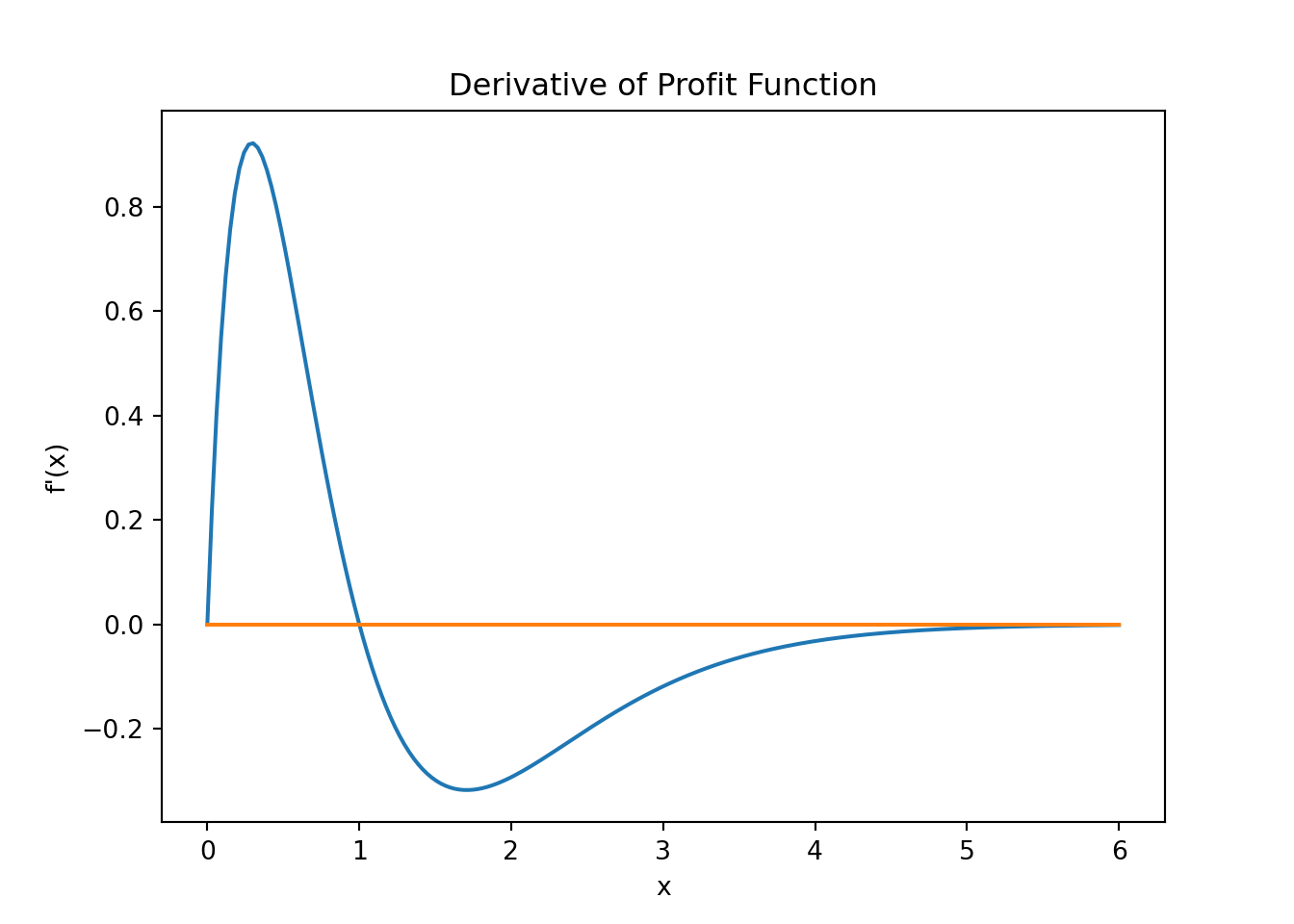

xmin <- 0.0
xmax <- 6.0
xv <- seq(from = xmin, to = xmax, length.out = 200)
dfx <- numeric(length(xv)) # Initialize a numeric vector

for (i in 1:length(xv)) {
    # The derivative value is in the second position of the output vector
    dfx[i] <- f_profit_plus_deriv(xv[i])[2]
}

plot(xv, dfx, type = "l", xlab = "x", ylab = "f'(x)", main = "Derivative of Profit Function")
abline(h = 0, col = "red")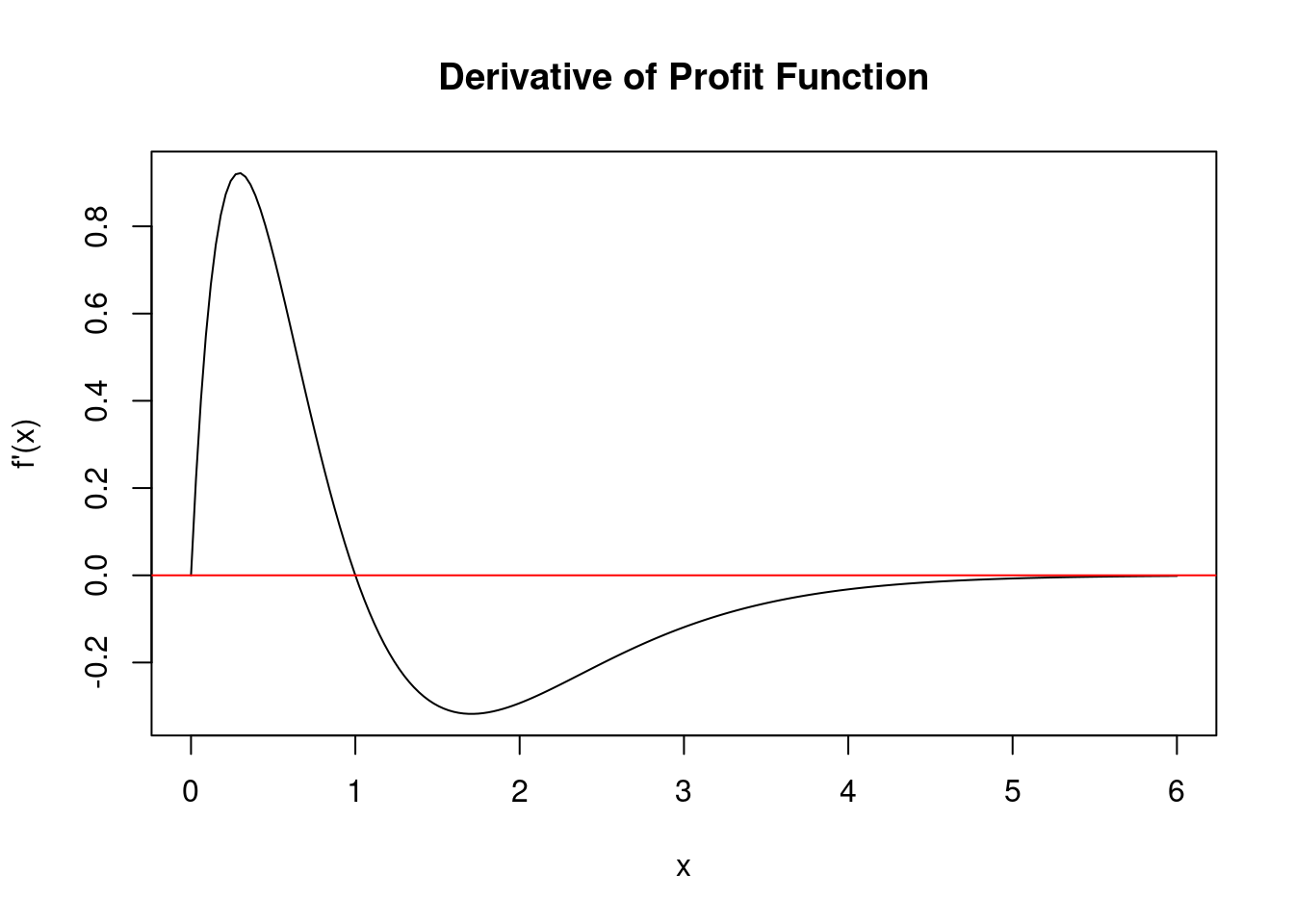

From this plot we see that the derivate function crosses the horizontal axis at and $x$ value of, well, one. So I gave it away, the maximum of the function is at $x = 1$ .

Let us pretend for a minute that we do not know that or are not entirely sure whether this is really our maximum value and let us therefore use the Newton algorithm from the previous chapter to make sure that the root of the derivative function is really at one. In order to implement the Newton method we basically look for the root of a first derivative so that $f^{'} (x) = 0$ .

Python Code
R Code

myOpt = 1.0
fmaxval = f_profit(myOpt)

xmin = 0.0
xmax = 6.0
xv = np.linspace(xmin, xmax, 200)
fx = np.zeros(len(xv),float) # define column vector
for i in range(len(xv)):
    fx[i] = f_profit_plus_deriv(xv[i])[0]

fig, ax = plt.subplots()
ax.plot(xv, fx)
ax.plot(xv, fmaxval*np.ones(len(xv)))
ax.axvline(x = myOpt, ymin=0.0, color='r', linestyle='--')
plt.show()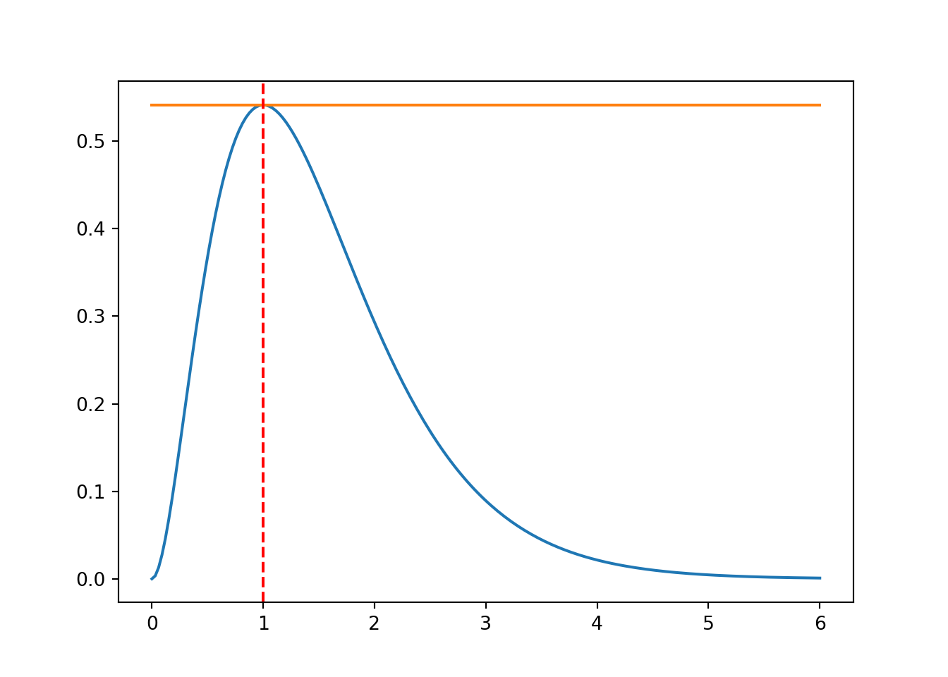

myOpt <- 1.0
fmaxval <- f_profit(myOpt)

xmin <- 0.0
xmax <- 6.0
xv <- seq(from = xmin, to = xmax, length.out = 200)
fx <- numeric(length(xv)) # Initialize a numeric vector

for (i in 1:length(xv)) {
    fx[i] <- f_profit_plus_deriv(xv[i])[1]
}

plot(xv, fx, type = "l", xlab = "x", ylab = "f(x)", main = "Profit Function and Maximum")
abline(h = fmaxval, col = "red")
abline(v = myOpt, col = "blue", lty = 2)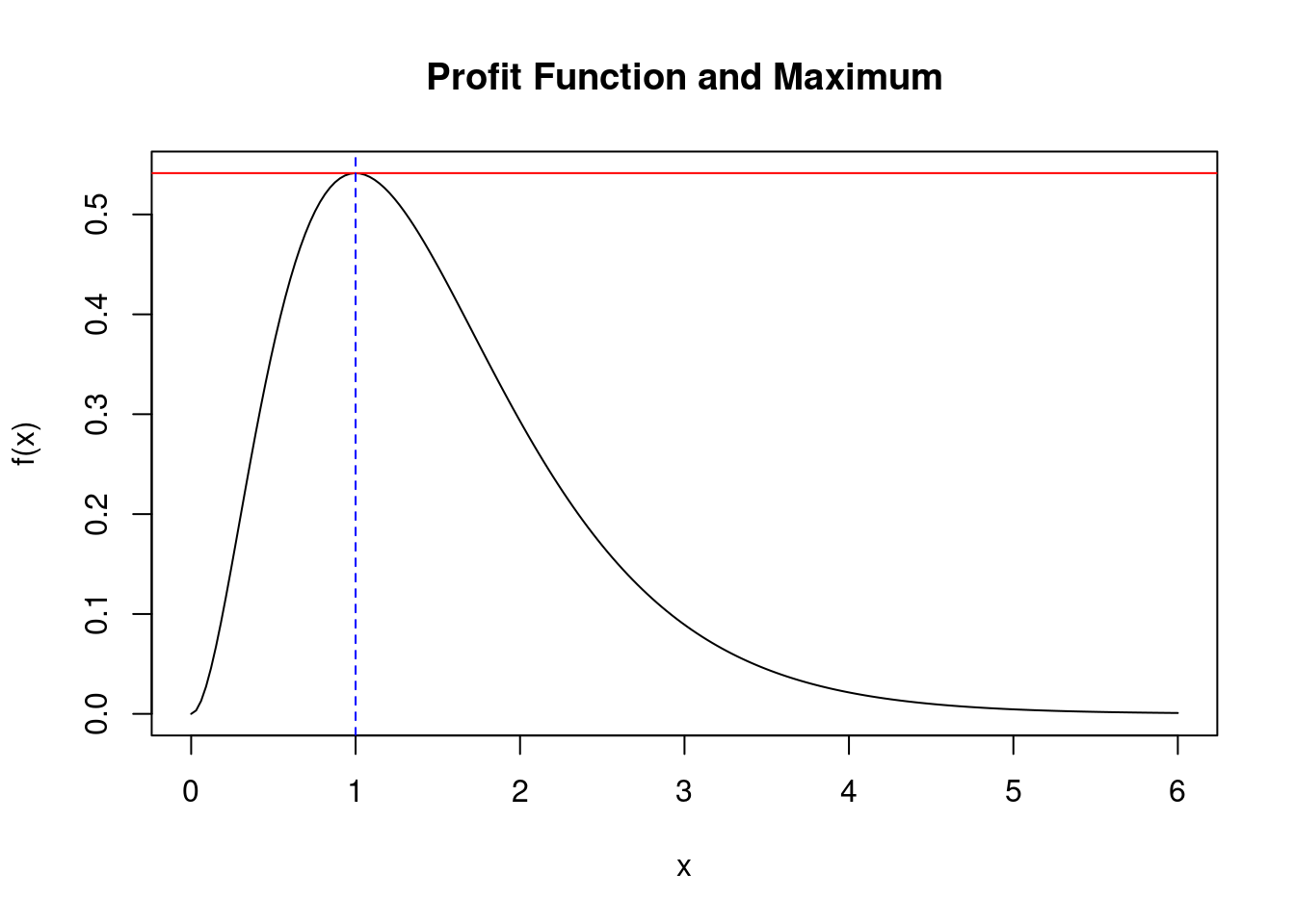

We then use the root finding algorithm from the previous chapter to find this point, or:

Note

Newthon-Raphson Root Finding Algorithm

$x_{n + 1} = x_{n} - \frac{f (x_{n})}{f^{'} (x_{n})}$

We have to adjust this of course because the function we search the foot for is already the first derivative of a function, so that we have:

$x_{n + 1} = x_{n} - \frac{f^{'} (x_{n})}{f^{″} (x_{n})}$

Python Code
R Code

def newton(f3, x0, tol = 1e-9, nmax = 100):
    # Newton's method for optimization, starting at x0
    # f3 is a function that given x returns the vector
    # (f(x), f'(x), f''(x)), for some f
    x = x0
    f3v = f3(x)
    n = 0
    while ((abs(f3v[1]) > tol) and (n < nmax)):
        # 1st derivative value is the second return value
        # 2nd derivative value is the third return value
        x = x - f3v[1]/f3v[2]
        f3v = f3(x)
        n = n + 1
    if (n == nmax):
        print("newton failed to converge")
    else:
        return(x)

newton <- function(f3, x0, tol = 1e-9, nmax = 100) {
    # Newton's method for optimization, starting at x0
    # f3 is a function that given x returns the vector
    # (f(x), f'(x), f''(x)), for some f
    x <- x0
    f3v <- f3(x)
    n <- 0
    while (abs(f3v[2]) > tol && n < nmax) {
        x <- x - f3v[2] / f3v[3]
        f3v <- f3(x)
        n <- n + 1
    }
    if (n == nmax) {
        cat("Newton failed to converge\n")
    } else {
        return(x)
    }
}

We next use these algorithms to find the maximum point of our function f_profit_plus_deriv and f_profit. Note that if we use the Newton algorithm we will need the first and second derivatives of the functions. This is why we use function f_profit_plus_deriv that returns f, f' and f'' via an array/vector as return value.

Python Code
R Code

print(" -----------------------------------")
print(" Newton results ")
print(" -----------------------------------")
print(newton(f_profit_plus_deriv, 0.25))
print(newton(f_profit_plus_deriv, 0.5))
print(newton(f_profit_plus_deriv, 0.75))
print(newton(f_profit_plus_deriv, 1.75))

 -----------------------------------
 Newton results 
 -----------------------------------
-1.25
1.0
0.9999999999980214
14.42367881581733

cat(" -----------------------------------\n")
cat(" Newton results \n")
cat(" -----------------------------------\n")
cat("Optimized value for x when starting at 0.25: ", newton(f_profit_plus_deriv, 0.25), "\n")
cat("Optimized value for x when starting at 0.5: ", newton(f_profit_plus_deriv, 0.5), "\n")
cat("Optimized value for x when starting at 0.75: ", newton(f_profit_plus_deriv, 0.75), "\n")
cat("Optimized value for x when starting at 1.75: ", newton(f_profit_plus_deriv, 1.75), "\n")

 -----------------------------------
 Newton results 
 -----------------------------------
Optimized value for x when starting at 0.25:  -1.25 
Optimized value for x when starting at 0.5:  1 
Optimized value for x when starting at 0.75:  1 
Optimized value for x when starting at 1.75:  14.42368

20.2.2 Golden Section Method

The golden-section method works in one dimension only, but does not need the derivatives of the function. However, the function still needs to be continuous. In order to determine whether there is a local maximum we need two starting points. For any midpoint $x_{m}$ we can then establish the following:

Note

If $x_{l} < x_{m} < x_{r}$ and

$f (x_{l}) \leq f (x_{m})$ and
$f (x_{r}) \leq f (x_{m})$ then there

must be a local maximum in the interval between $[x_{l}, x_{r}] .$

Figure 20.1 illustrates this case with a maximum point. A similar “statement” can be derived for a minimum, but we focus on maximums for now.

Figure 20.1: Maximization using the Golden Ratio Algorithm

The method operates by successively narrowing the range of values on the specified interval $x_{l}$ to $x_{r}$ by “moving in” the brackets (or boundary points) and thereby narrowing the interval around the maximum point. This is very similar to the bisection algorithm we saw in the last chapter.

Figure 20.2: Maximization using the Golden Ratio Algorithm

Given that the function value $f (y)$ is below the function value $f (x_{m})$ we conclude the maximum must be in the interval $[x_{l}, y]$ (as opposed to the equally large interval $[x_{m}, x_{r}]$ ). We therefore move the “right” bracket inwards and declare value $y$ as our new upper bound x-value $x_{r}$ . The algorithm then proceeds with the newly established (smaller) interval and finds a new $y$ and $f (y)$ value until the lower bracket $x_{l}$ and upper bracket $x_{r}$ are very close to each other.

The Golden Section Search then proceeds as follows:

Start with $x_{l} < x_{m} < x_{r}$ such that $f (x_{l}) \leq f (x_{m})$ and $f (x_{r}) \leq f (x_{m})$ .

If $x_{r} - x_{l} \leq ϵ$ then stop

If $x_{r} - x_{m} > x_{m} - x_{l}$ then do $(a)$ otherwise do $(b)$

Choose a point $y \in (x_{m}, x_{r})$ If $f (y) \geq f (x_{m})$ then put $x_{l} = x_{m}$ and $x_{m} = y$ otherwise put $x_{r} = y$

Choose a point $y \in (x_{l}, x_{m})$ If $f (y) \geq f (x_{m})$ then put $x_{r} = x_{m}$ and $x_{m} = y$ otherwise put $x_{l} = y$

Go back to step 1

Note that we have not yet explained how to choose $y$ ! Let us do a quick detour first but we will come back to it after this note.

Note

In mathematics, two quantities $a$ and $b$ are in the golden ratio if their ratio is the same as the ratio of their sum to the larger of the two quantities. Assume $a > b$ then the ratio:

$\frac{a}{b} = \frac{a + b}{a} = φ$

Figure 20.3 illustrates this geometric relationship.

Figure 20.3: Line segments in the golden ratio

The golden ratio is the solution to:

${(\frac{a}{b})}^{2} - (\frac{a}{b}) - 1 = 0,$

so that

$(\frac{a}{b}) = φ = \frac{1 + \sqrt{5}}{2} .$

Remember that the solution to a quadratic equation of the form $a \times x^{2} + b \times x + c = 0$ is $x_{1, 2} = \frac{- b \pm \sqrt{b^{2} - 4 \times a \times c}}{2 a}$

In the quadratic above we therefore have: $1 \times {(\frac{a}{b})}^{2} - 1 \times (\frac{a}{b}) - 1 = 0,$

so that the solution for the “variable” $\frac{a}{b}$ becomes ${(\frac{a}{b})}_{1, 2} = \frac{- (- 1) \pm \sqrt{(- 1)^{2} - 4 \times 1 \times (- 1)}}{2 \times 1},$

which can be simplified to

${(\frac{a}{b})}_{1, 2} = \frac{1 \pm \sqrt{5}}{2} = 1.618033988 . . .,$

We only use the “positive” of the two possible solutions.

The Golden Rule search method uses this principle and attempts to narrow a lower and upper bracket around a maximum by sequentially ruling out intervals on the x-axis where the maximum cannot be. These successively narrower intervals follow a specific pattern where the ratio of the three intervals (defined by 4 points on the x-axis) stays constant as shown in Figure 20.4. This ensures stable convergence properties.

Independent of how you initially choose $x_{m}$ , the interval ratio that is maintained in this way is eventually fixed at $φ : 1 : φ$ , where $φ$ is the golden ratio (the number from the note box above). These ratios are maintained for each iteration and can be shown to follow the “optimal” rate of convergence.

Figure 20.4 illustrates this for a maximization problem which we set up according to the golden ratio algorithm. The graph shows that the ratio of the intervals I,II, and III follow the fixed ratio established by the golden rule section search.

Figure 20.4: Maximization using the Golden Ratio Algorithm

In the picture we started with 3! candidate values $x_{l}$ and $x_{r}$ as the outer boundary points that need to contain the maximum and one suitably chosen point in the interval $x_{m}$ .

The issue is now how to choose point $y$ . We pick the new candidate point $y$ in the graph to maintain this fixed ratio so that if the new bracketing interval is $[x_{l}, y]$ then the ratios satisfy: $\frac{a}{c} = \frac{b}{a},$ while if the new bracketing interval is $[x_{m}, x_{r}]$ then the ratios satisfy: $\frac{b - c}{c} = \frac{b}{a} .$

We can now go back to the note box of the Golden Rule and establish that the ratio $\frac{b}{a} = φ$ by solving the two equations above for $\frac{b}{a}$ . Eliminating $c$ from the 2-equation system results in ${(\frac{b}{a})}^{2} - (\frac{b}{a}) - 1 = 0,$

which can be solved for:

${(\frac{b}{a})}_{1, 2} = φ = \frac{1 \pm \sqrt{5}}{2} = 1.618033988 . . .$

Note that here the fraction $\frac{b}{a}$ is reversed (compared to the discussion in the note box for the golden rule) because in our graph $b > a$ .

From the solution to this problem we also get $a = b - c$ and $c = b / (1 + φ)$ which we can use to calculate a candidate point $y = x_{m} + c = x_{m} + (x_{r} - x_{m}) / (1 + φ),$ and expression you will see in the final algorithm below.

Note

Start with $x_{l} < x_{m} < x_{r}$ such that

$f (x_{l}) \leq (x_{m})$

and

$f (x_{r}) \leq f (x_{m})$

and the golden ratio

$φ = \frac{1 + \sqrt{5}}{2} .$

In the algorithm we then check the following:

If $x_{r} - x_{l} \leq ϵ$ then stop

If $x_{r} - x_{m} > x_{m} - x_{l}$ then do $(a)$ otherwise do $(b)$

Let $y = x_{m} + (x_{r} - x_{m}) / (1 + φ)$ if $f (y) \geq f (x_{m})$ then put $x_{l} = x_{m}$ and $x_{m} = y$ otherwise put $x_{r} = y$

Let $y = x_{m} + (x_{m} - x_{l}) / (1 + φ)$ if $f (y) \geq f (x_{m})$ then put $x_{r} = x_{m}$ and $x_{m} = y$ otherwise put $x_{l} = y$

Go back to step 1

Python Code
R Code

def gsection(ftn, xl, xm, xr, tol = 1e-9):
    # applies the golden-section algorithm to maximise ftn
    # we assume that ftn is a function of a single variable
    # and that x.l < x.m < x.r and ftn(x.l), ftn(x.r) <= ftn(x.m)
    #
    # the algorithm iteratively refines x.l, x.r, and x.m and
    # terminates when x.r - x.l <= tol, then returns x.m
    # golden ratio plus one
    gr1 = 1 + (1 + np.sqrt(5))/2
    #
    # successively refine x.l, x.r, and x.m
    fl = ftn(xl)
    fr = ftn(xr)
    fm = ftn(xm)
    while ((xr - xl) > tol):
        if ((xr - xm) > (xm - xl)):
            y = xm + (xr - xm)/gr1
            fy = ftn(y)
            if (fy >= fm):
                xl = xm
                fl = fm
                xm = y
                fm = fy
            else:
                xr = y
                fr = fy
        else:
            y = xm - (xm - xl)/gr1
            fy = ftn(y)
            if (fy >= fm):
                xr = xm
                fr = fm
                xm = y
                fm = fy
            else:
                xl = y
                fl = fy
    return(xm)

gsection <- function(ftn, xl, xm, xr, tol = 1e-9) {
  # Applies the golden-section algorithm to maximize ftn
  # Assumes that ftn is a function of a single variable
  # and that xl < xm < xr and ftn(xl), ftn(xr) <= ftn(xm)
  #
  # The algorithm iteratively refines xl, xr, and xm and
  # terminates when xr - xl <= tol, then returns xm
  # Golden ratio plus one
  gr1 <- 1 + (1 + sqrt(5))/2
  #
  # Successively refine xl, xr, and xm
  fl <- ftn(xl)
  fr <- ftn(xr)
  fm <- ftn(xm)
  while ((xr - xl) > tol) {
    if ((xr - xm) > (xm - xl)) {
      y <- xm + (xr - xm)/gr1
      fy <- ftn(y)
      if (fy >= fm) {
        xl <- xm
        fl <- fm
        xm <- y
        fm <- fy
      } else {
        xr <- y
        fr <- fy
      }
    } else {
      y <- xm - (xm - xl)/gr1
      fy <- ftn(y)
      if (fy >= fm) {
        xr <- xm
        fr <- fm
        xm <- y
        fm <- fy
      } else {
        xl <- y
        fl <- fy
      }
    }
  }
  return(xm)
}

The Golden section algorithm does not require the derivates of the function, so we just call the f_profit function that only returns the functional value.

Python Code
R Code

print(" -----------------------------------")
print(" Golden section results ")
print(" -----------------------------------")
myOpt = gsection(f_profit, 0.1, 0.25, 1.3)
print(gsection(f_profit, 0.1, 0.25, 1.3))
print(gsection(f_profit, 0.25, 0.5, 1.7))
print(gsection(f_profit, 0.6, 0.75, 1.8))
print(gsection(f_profit, 0.0, 2.75, 5.0))

 -----------------------------------
 Golden section results 
 -----------------------------------
1.0000000117853984
1.0000000107340477
0.9999999921384167
1.0000000052246139

# Print results using gsection
cat(" -----------------------------------\n")
cat(" Golden section results \n")
cat(" -----------------------------------\n")
myOpt <- gsection(f_profit, 0.1, 0.25, 1.3)
cat("Optimal value for myOpt: ", myOpt, "\n")
cat("Optimal value for (0.1, 0.25, 1.3): ", gsection(f_profit, 0.1, 0.25, 1.3), "\n")
cat("Optimal value for (0.25, 0.5, 1.7): ", gsection(f_profit, 0.25, 0.5, 1.7), "\n")
cat("Optimal value for (0.6, 0.75, 1.8): ", gsection(f_profit, 0.6, 0.75, 1.8), "\n")
cat("Optimal value for (0.0, 2.75, 5.0): ", gsection(f_profit, 0.0, 2.75, 5.0), "\n")

 -----------------------------------
 Golden section results 
 -----------------------------------
Optimal value for myOpt:  1 
Optimal value for (0.1, 0.25, 1.3):  1 
Optimal value for (0.25, 0.5, 1.7):  1 
Optimal value for (0.6, 0.75, 1.8):  1 
Optimal value for (0.0, 2.75, 5.0):  1

20.2.3 Use Built-In Method to Maximize Function

Finally, we can also use a built in function minimizer. The built in function fmin is in the scipy.optimize library. We need to import it first. So if we want to maximize our function we have to define it as a negated function, that is:

$g (x) = - f (x)$

then

$m i n g (x)$

is the same as

$m a x f (x) .$

Since we want to find the maximum of the function, we need to "trick" the minimization algorithm. We therefore need to redefine the function as

Python Code
R Code

def f_profitNeg(x):
    # gamma(2,3) density
    if (x < 0):
        return (0)
    if (x == 0):
        return (np.nan)
    y = np.exp(-2*x)
    return (-(4 * x**2 * y))

f_profitNeg <- function(x) {
  if (x < 0) {
    return(0)
  }
  if (x == 0) {
    return(NA)
  }
  y <- exp(-2 * x)
  return(-(4 * x^2 * y))
}

Here we simply return negative values of this function. If we now minimize this function, we actually maximize the original function

$f (x) = 4 x^{2} e^{- 2 x}$

Python Code
R Code

from scipy.optimize import fmin

print(" -----------------------------------")
print(" fmin results ")
print(" -----------------------------------")
print(fmin(f_profitNeg, 0.25))
print(fmin(f_profitNeg, 0.5))
print(fmin(f_profitNeg, 0.75))
print(fmin(f_profitNeg, 1.75))

 -----------------------------------
 fmin results 
 -----------------------------------
Optimization terminated successfully.
         Current function value: -0.541341
         Iterations: 18
         Function evaluations: 36
[1.]
Optimization terminated successfully.
         Current function value: -0.541341
         Iterations: 16
         Function evaluations: 32
[1.]
Optimization terminated successfully.
         Current function value: -0.541341
         Iterations: 14
         Function evaluations: 28
[0.99997559]
Optimization terminated successfully.
         Current function value: -0.541341
         Iterations: 16
         Function evaluations: 32
[1.00001221]

In R, you can use the optim function for optimization tasks similar to fmin in Python. The par parameter is the initial guess for the optimum, and fn is the function to be minimized. The results are accessed through $par.

# Example usage
print(" -----------------------------------")
print(" optim results ")
print(" -----------------------------------")

result1 <- optim(par = 0.25, fn = f_profitNeg)

Warning in optim(par = 0.25, fn = f_profitNeg): one-dimensional optimization by Nelder-Mead is unreliable:
use "Brent" or optimize() directly

print(result1$par)

result2 <- optim(par = 0.5, fn = f_profitNeg)

Warning in optim(par = 0.5, fn = f_profitNeg): one-dimensional optimization by Nelder-Mead is unreliable:
use "Brent" or optimize() directly

print(result2$par)

result3 <- optim(par = 0.75, fn = f_profitNeg)

Warning in optim(par = 0.75, fn = f_profitNeg): one-dimensional optimization by Nelder-Mead is unreliable:
use "Brent" or optimize() directly

print(result3$par)

result4 <- optim(par = 1.75, fn = f_profitNeg)

Warning in optim(par = 1.75, fn = f_profitNeg): one-dimensional optimization by Nelder-Mead is unreliable:
use "Brent" or optimize() directly

print(result4$par)

[1] " -----------------------------------"
[1] " optim results "
[1] " -----------------------------------"
[1] 1
[1] 1
[1] 1.000049
[1] 0.9999268

20.3 Finding the Root of a Function using Minimization

In a previous chapter on root searching of a function we used various methods like the built in fsolve or root functions from the scipy.optimize library. Here's the example from the Root finding chapter again:

The example function for which we calculate the root, i.e., find $x$ so that $f (x) = 0$ is defined as:

Python Code
R Code

def func(x):
    s = np.log(x) - np.exp(-x)  # function: f(x)
    return s

func <- function(x) {
  s <- log(x) - exp(-x)  # function: f(x)
  return(s)
}

We can solve for the zero (root) position with:

Python Code
R Code

from scipy.optimize import root

guess = 2
result = root(func, guess) # starting from x = 2
print(" ")
print(" -------------- Root ------------")
myroot = result.x  # Grab number from result dictionary
print("The root of d_func is at {}".format(myroot))
print("The max value of the function is {}".format(myOpt))

 
 -------------- Root ------------
The root of d_func is at [1.30979959]
The max value of the function is 1.0000000117853984

library(rootSolve)

guess <- 2
result <- uniroot(func, interval = c(0.7, guess))  # Starting from x = 2

cat(" \n")
cat(" -------------- Root ------------\n")
myroot <- result$root  # Extract the root value
cat("The root of d_func is at", myroot, "\n")
cat("The max value of the function is", myOpt, "\n")

 
 -------------- Root ------------
The root of d_func is at 1.309803 
The max value of the function is 1

In this section we set up the root finding problem as an optimization problem. In order to do this we change the return value of the function slightly to

$residual-error = (f (x) - 0)^{2} .$

So we are trying to find the value of x so that the residual error between $f (x)$ and its target value of $0$ is as small as possible. The new function is defined as:

Python Code
R Code

def func_root_min(x):
    s = np.log(x) - np.exp(-x)  # function: f(x)
    return (s**2)

func_root_min <- function(x) {
  s <- log(x) - exp(-x)  # function: f(x)
  return(s^2)
}

We now invoke a minimizing algorithm to find this value of $x$

Python Code
R Code

from scipy.optimize import minimize

guess = 2 # starting guess x = 2
result_min = minimize(func_root_min, guess, method='Nelder-Mead')

print(" ")
print("-------------- Root ------------")
myroot = result_min.x  # Grab number from result dictionary
print("The root of func is at {}".format(myroot))

 
-------------- Root ------------
The root of func is at [1.30976562]

# Starting guess
guess <- 2

# Perform the minimization
result_min <- optim(guess, func_root_min, method = "Nelder-Mead")

Warning in optim(guess, func_root_min, method = "Nelder-Mead"): one-dimensional optimization by Nelder-Mead is unreliable:
use "Brent" or optimize() directly

cat("\n")
cat("-------------- Root ------------\n")
myroot <- result_min$par  # Extract the minimizer from the result
cat(paste("The root of func is at", myroot), "\n")


-------------- Root ------------
The root of func is at 1.309765625

20.4 Multivariate Optimization

20.4.1 Function

Here we want to optimize the following function f3

Python Code
R Code

def f3simple(x):
    a = x[0]**2/2.0 - x[1]**2/4.0
    b = 2*x[0] - np.exp(x[1])
    f = np.sin(a)*np.cos(b)
    return(f)

f3simple <- function(x) {
  a <- x[1]^2/2 - x[2]^2/4
  b <- 2*x[1] - exp(x[2])
  f <- sin(a) * cos(b)
  return(f)
}

Its negative version:

Python Code
R Code

def f3simpleNeg(x):
    a = x[0]**2/2.0 - x[1]**2/4.0
    b = 2*x[0] - np.exp(x[1])
    f = -np.sin(a)*np.cos(b)
    return(f)

f3simpleNeg <- function(x) {
  a <- x[1]^2/2 - x[2]^2/4
  b <- 2*x[1] - exp(x[2])
  f <- -sin(a) * cos(b)
  return(f)
}

And the version that returns $f (x)$ , $f^{'} (x)$ (i.e., the gradient), and $f^{″} (x)$ (i.e., the Hessian matrix):

Python Code
R Code

def f3(x):
    a = x[0]**2/2.0 - x[1]**2/4.0
    b = 2*x[0] - np.exp(x[1])
    f = np.sin(a)*np.cos(b)
    f1 = np.cos(a)*np.cos(b)*x[0] - np.sin(a)*np.sin(b)*2
    f2 = -np.cos(a)*np.cos(b)*x[1]/2 + np.sin(a)*np.sin(b)*np.exp(x[1])
    f11 = -np.sin(a)*np.cos(b)*(4 + x[0]**2) + np.cos(a)*np.cos(b) \
        - np.cos(a)*np.sin(b)*4*x[0]
    f12 = np.sin(a)*np.cos(b)*(x[0]*x[1]/2.0 + 2*np.exp(x[1])) \
        + np.cos(a)*np.sin(b)*(x[0]*np.exp(x[1]) + x[1])
    f22 = -np.sin(a)*np.cos(b)*(x[1]**2/4.0 + np.exp(2*x[1])) \
        - np.cos(a)*np.cos(b)/2.0 - np.cos(a)*np.sin(b)*x[1]*np.exp(x[1]) \
        + np.sin(a)*np.sin(b)*np.exp(x[1])
    # Function f3 returns: f(x), f'(x), and f''(x)
    return (f, np.array([f1, f2]), np.array([[f11, f12], [f12, f22]]))

f3 <- function(x) {
  a <- x[1]^2/2 - x[2]^2/4
  b <- 2*x[1] - exp(x[2])
  f <- sin(a) * cos(b)
  f1 <- cos(a) * cos(b) * x[1] - sin(a) * sin(b) * 2
  f2 <- -cos(a) * cos(b) * x[2]/2 + sin(a) * sin(b) * exp(x[2])
  f11 <- -sin(a) * cos(b) * (4 + x[1]^2) + cos(a) * cos(b) - cos(a) * sin(b) * 4 * x[1]
  f12 <- sin(a) * cos(b) * (x[1] * x[2]/2 + 2 * exp(x[2])) + cos(a) * sin(b) * (x[1] * exp(x[2]) + x[2])
  f22 <- -sin(a) * cos(b) * (x[2]^2/4 + exp(2 * x[2])) - cos(a) * cos(b)/2 - cos(a) * sin(b) * x[2] * exp(x[2]) + sin(a) * sin(b) * exp(x[2])
  # Function f3 returns: f(x), f'(x), and f''(x)
  return (list(f, c(f1, f2), matrix(c(f11, f12, f12, f22), nrow = 2, ncol = 2)))
}

We next plot the function:

Python Code
R Code

X = np.arange(-3, 3, .1)
Y = np.arange(-3, 3, .1)
X, Y = np.meshgrid(X, Y)

Z = np.zeros((len(X),len(Y)),float)
for i in range(len(X)):
    for j in range(len(Y)):
        Z[i][j] = f3simple([X[i][j],Y[i][j]])

ax = plt.figure(figsize=(6, 7)).add_subplot(projection='3d')
ax.plot_surface(X, Y, Z, rstride=1, cstride=1, \
    cmap=plt.cm.jet, linewidth=0, antialiased=False)
plt.show()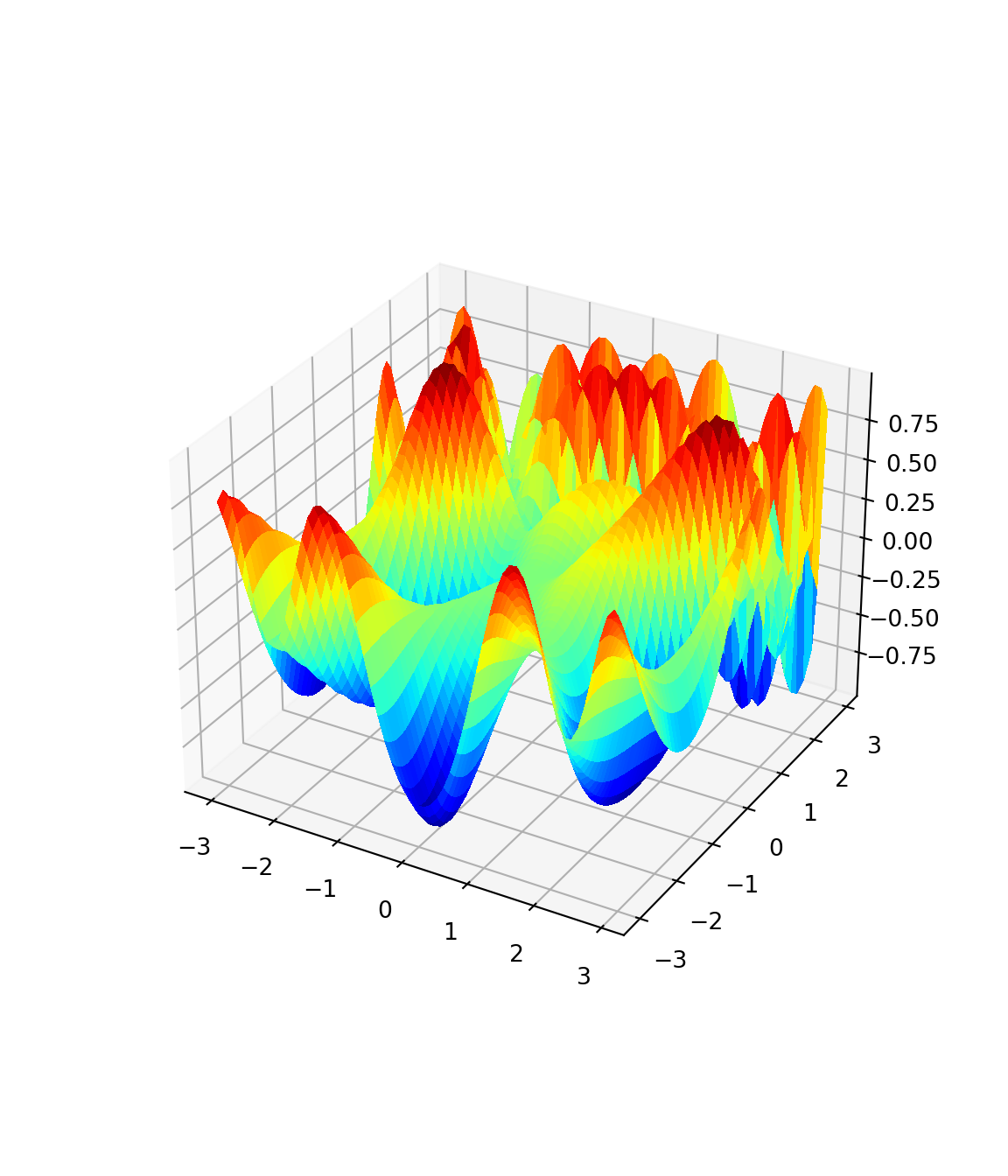

# Load the rgl package
library(rgl)

# Define the range for X and Y values
X <- seq(-3, 3, by = 0.1)
Y <- seq(-3, 3, by = 0.1)

# Create a grid of X and Y values
XY <- expand.grid(X, Y)

# Calculate Z values using f3simple
Z <- sapply(1:nrow(XY), function(i) {
  f3simple(c(XY[i, 1], XY[i, 2]))
})

# Reshape Z into a matrix
Z_matrix <- matrix(Z, nrow = length(X), ncol = length(Y), byrow = TRUE)

# Create a 3D plot
plot3d(X, Y, Z_matrix, type = "surface", color = "jet")

# Adjust plot settings if needed
rgl.postscript("3d_plot.png", fmt = "png")

Error in rgl.enum(postscripttype, ps = 0, eps = 1, tex = 2, pdf = 3, svg = 4, : Symbolic value must be chosen from: c("ps", "eps", "tex", "pdf", "svg", "pgf")

# To rotate the plot interactively in RStudio, use:
# rglwidget()

def newtonMult(f3, x0, tol = 1e-9, nmax = 100):
    # Newton's method for optimization, starting at x0
    # f3 is a function that given x returns the list
    # {f(x), grad f(x), Hessian f(x)}, for some f
    x = x0
    f3x = f3(x)
    n = 0
    while ((max(abs(f3x[1])) > tol) and (n < nmax)):
        x = x - np.linalg.solve(f3x[2], f3x[1])
        f3x = f3(x)
        n = n + 1
    if (n == nmax):
        print("newton failed to converge")
    else:
        return(x)

newtonMult <- function(f3, x0, tol = 1e-9, nmax = 100) {
  # Newton's method for optimization, starting at x0
  # f3 is a function that given x returns the list
  # {f(x), grad f(x), Hessian f(x)}, for some f
  x <- x0
  f3x <- f3(x)
  n <- 0
  while (max(abs(f3x[[2]])) > tol && n < nmax) {
    x <- x - solve(f3x[[3]], f3x[[2]])
    f3x <- f3(x)
    n <- n + 1
  }
  if (n == nmax) {
    cat("newton failed to converge\n")
  } else {
    return(x)
  }
}

# Example usage:
# x0 <- c(0, 0)  # Initial guess
# result <- newtonMult(f3, x0)
# print(result)

Compare the Newton method with the built in fmin method in scipy.optimize. We use various starting values to see whether we can find more than one optimum.

Python Code
R Code

from scipy.optimize import fmin

for x0 in np.arange(1.4, 1.6, 0.1):
    for y0 in np.arange(0.4, 0.7, 0.1):
        # This algorithm requires f(x), f'(x), and f''(x)
        print("Newton: f3  " + str([x0,y0]) + ' --> ' + str(newtonMult(f3, \
            np. array([x0,y0]))))

        print("fmin: f3 " + str([x0,y0]) + ' --> ' \
            + str(fmin(f3simpleNeg, np.array([x0,y0]))))

        print(" ----------------------------------------- ")

Newton: f3  [1.4, 0.4] --> [ 0.04074437 -2.50729047]
Optimization terminated successfully.
         Current function value: -1.000000
         Iterations: 47
         Function evaluations: 89
fmin: f3 [1.4, 0.4] --> [2.0307334  1.40155445]
 ----------------------------------------- 
Newton: f3  [1.4, 0.5] --> [0.11797341 3.34466147]
Optimization terminated successfully.
         Current function value: -1.000000
         Iterations: 50
         Function evaluations: 93
fmin: f3 [1.4, 0.5] --> [2.03072555 1.40154756]
 ----------------------------------------- 
Newton: f3  [1.4, 0.6] --> [-1.5531627  6.0200129]
Optimization terminated successfully.
         Current function value: -1.000000
         Iterations: 43
         Function evaluations: 82
fmin: f3 [1.4, 0.6] --> [2.03068816 1.40151998]
 ----------------------------------------- 
Newton: f3  [1.5, 0.4] --> [2.83714224 5.35398196]
Optimization terminated successfully.
         Current function value: -1.000000
         Iterations: 48
         Function evaluations: 90
fmin: f3 [1.5, 0.4] --> [2.03067611 1.40149298]
 ----------------------------------------- 
Newton: f3  [1.5, 0.5] --> [ 0.04074437 -2.50729047]
Optimization terminated successfully.
         Current function value: -1.000000
         Iterations: 42
         Function evaluations: 82
fmin: f3 [1.5, 0.5] --> [2.03071509 1.40155165]
 ----------------------------------------- 
Newton: f3  [1.5, 0.6] --> [9.89908350e-10 1.36639196e-09]
Optimization terminated successfully.
         Current function value: -1.000000
         Iterations: 43
         Function evaluations: 82
fmin: f3 [1.5, 0.6] --> [2.0307244  1.40153761]
 ----------------------------------------- 
Newton: f3  [1.6, 0.4] --> [-0.55841026 -0.78971136]
Optimization terminated successfully.
         Current function value: -1.000000
         Iterations: 47
         Function evaluations: 88
fmin: f3 [1.6, 0.4] --> [2.0307159  1.40150964]
 ----------------------------------------- 
Newton: f3  [1.6, 0.5] --> [-0.29022131 -0.23047994]
Optimization terminated successfully.
         Current function value: -1.000000
         Iterations: 44
         Function evaluations: 80
fmin: f3 [1.6, 0.5] --> [2.03074135 1.40151521]
 ----------------------------------------- 
Newton: f3  [1.6, 0.6] --> [-1.55294692 -3.33263763]
Optimization terminated successfully.
         Current function value: -1.000000
         Iterations: 42
         Function evaluations: 80
fmin: f3 [1.6, 0.6] --> [2.03069759 1.40155333]
 -----------------------------------------

for (x0 in seq(1.4, 1.6, by = 0.1)) {
  for (y0 in seq(0.4, 0.7, by = 0.1)) {
    # This algorithm requires f(x), f'(x), and f''(x)
    cat("Newton: f3  ", c(x0, y0), " --> ", newtonMult(f3, c(x0, y0)), "\n")

    result_min <- optim(c(x0, y0), f3simpleNeg)
    cat("optim: f3 ", c(x0, y0), " --> ", result_min$par, "\n")

    cat(" -----------------------------------------\n")
  }
}

Newton: f3   1.4 0.4  -->  0.04074437 -2.50729 
optim: f3  1.4 0.4  -->  2.03071 1.401523 
 -----------------------------------------
Newton: f3   1.4 0.5  -->  0.1179734 3.344661 
optim: f3  1.4 0.5  -->  2.03071 1.401541 
 -----------------------------------------
Newton: f3   1.4 0.6  -->  -1.553163 6.020013 
optim: f3  1.4 0.6  -->  2.030687 1.401515 
 -----------------------------------------
Newton: f3   1.4 0.7  -->  -0.7731558 -3.709705 
optim: f3  1.4 0.7  -->  2.030682 1.401522 
 -----------------------------------------
Newton: f3   1.5 0.4  -->  2.837142 5.353982 
optim: f3  1.5 0.4  -->  2.030681 1.401512 
 -----------------------------------------
Newton: f3   1.5 0.5  -->  0.04074437 -2.50729 
optim: f3  1.5 0.5  -->  2.030674 1.401523 
 -----------------------------------------
Newton: f3   1.5 0.6  -->  9.899083e-10 1.366392e-09 
optim: f3  1.5 0.6  -->  2.030682 1.401527 
 -----------------------------------------
Newton: f3   1.5 0.7  -->  2.585751e-17 3.053722e-17 
optim: f3  1.5 0.7  -->  2.030694 1.401503 
 -----------------------------------------
Newton: f3   1.6 0.4  -->  -0.5584103 -0.7897114 
optim: f3  1.6 0.4  -->  2.030685 1.401521 
 -----------------------------------------
Newton: f3   1.6 0.5  -->  -0.2902213 -0.2304799 
optim: f3  1.6 0.5  -->  2.030696 1.401522 
 -----------------------------------------
Newton: f3   1.6 0.6  -->  -1.552947 -3.332638 
optim: f3  1.6 0.6  -->  2.030685 1.401525 
 -----------------------------------------
Newton: f3   1.6 0.7  -->  6.886167e-10 8.21652e-10 
optim: f3  1.6 0.7  -->  2.03068 1.401506 
 -----------------------------------------

Key Concepts and Summary

Introduction to basic optimization algorithms

Self-check questions

Solve the following maximization problem.