24  Growth Models

Chapter Learning Objectives
  • Solow Growth Model

25 The Solow Growth Models

The Solow growth model is an economic framework that explains the long-run economic growth and its implications. Developed by Robert Solow, this model focuses on the relationships between capital accumulation, population growth, and technological progress as drivers of economic growth.

25.1 Basic Model Structure

The model consists of the following key components:

  • Production Function: It describes how an economy converts inputs (capital and labor) into output.

  • Capital Accumulation: The process of investment in capital goods, determining the economy’s capital stock over time.

  • Population Growth: Changes in the labor force due to births and deaths.

  • Technological Progress: Enhancements in technology or productivity growth.

The production function expresses the relationship between the economy’s output and the inputs of capital (\(K_t\)) and labor (\(N_t\)):

\[ Y_t = A \times F(K_t, N_t) \]

  1. The capital accumulation equation:

The change in capital per worker over time is defined by the investment in new capital (\(sY_t\)) and the depreciation of existing capital (\(\delta K_t\)):

\[ \Delta K_t = sY_t - \delta K_t \]

  1. The capital law of motion:

This equation characterizes the dynamic accumulation of capital per worker in each period:

\[ K_{t+1} = (1 - \delta)K_t + sF(K_t, N_t) \]

We can express this in per capita terms by dividing both sides with \(N_t\) so we get \[ k_{t+1} \times (1+n) = s \times A \times F(k_t, 1) + (1 - \delta)k_t \]

where \(k=\frac{K}{N}\). After dividing by \(1+n\) and using $f(k_t)=F(k_t,1) we get the per capita capital law of motion:

\[ k_{t+1} = \frac{s \times A \times f(k_t)}{1+n} + \frac{(1 - \delta)}{1+n} \times k_t \]

  1. The steady-state condition:

The steady state occurs when the capital per worker no longer changes over time:

\[ k_{t+1} = k_t = k^* \]

  1. The steady-state level of capital per worker:

Using a Cobb-Douglas production function

\[ Y_t = A \times F(K_t, N_t) = A \times K_t^\alpha N_t^{(1-\alpha)}\]

and expressing it on a per capita basis as:

\[ y_t = A \times k_t^\alpha. \]

We then use the law of motion of per-capita-capital:

\[ k_{t+1} = \frac{s \times A \times k_t^\alpha}{1+n} + \frac{(1 - \delta)}{1+n} \times k_t \]

and impose the steady state condition \(k_{t+1}=k_t=k^*\) so that the law of motion becomes

\[ k^* = \frac{s \times A \times (k^*)^\alpha}{1+n} + \frac{(1 - \delta)}{1+n} \times k^*. \]

We can now solve this for steady-state capital per capita \(k^*\):

\[ k^* = \left(\frac{s \times A}{n+\delta}\right)^{\frac{1}{1-\alpha}} \]
25.2 Python Code for Plotting Capital Law of Motion and Steady State

Below is the Python code to visualize the capital law of motion and the steady state of per capita capital:

import numpy as np
import matplotlib.pyplot as plt

# Parameters
A = 1       # TFP
s = 0.2     # savings rate
alpha = 0.3  # output elasticity of capital
n = 0.02  # population growth rate
d = 0.05  # depreciation rate

# Capital law of motion
def f_kprime(k):
    return s *A * k**alpha/(1.+n) + (1-d)/(1+n)*k

# Steady-state capital per worker
kstar = (s*A/(n+d))**(1/(1-alpha))

# Time and capital per worker
tv = np.arange(0, 100, 1)

kv = np.zeros(len(tv))
kprimev = np.zeros(len(tv))

kv[0] = 3.0  # initial capital per worker
kprimev[0] = f_kprime(kv[0]) # capital tomorrow

for t in range(1, len(tv)):
    kv[t] = kprimev[t-1]
    kprimev[t] = f_kprime(kv[t])

print(kv[1:5])
[3.06674297 3.13071114 3.19199422 3.2506822 ]
# Parameters
A <- 1       # TFP
s <- 0.2     # savings rate
alpha <- 0.3  # output elasticity of capital
n <- 0.02  # population growth rate
d <- 0.05  # depreciation rate

# Capital law of motion
f_kprime <- function(k) {
  return(s * A * k^alpha / (1 + n) + (1 - d) / (1 + n) * k)
}

# Steady-state capital per worker
kstar <- (s * A / (n + d))^(1 / (1 - alpha))

# Time and capital per worker
tv <- seq(0, 100, 1)

kv <- rep(0, length(tv))
kprimev <- rep(0, length(tv))

kv[1] <- 3.0  # initial capital per worker
kprimev[1] <- f_kprime(kv[1])  # capital tomorrow

for (t in 2:length(tv)) {
  kv[t] <- kprimev[t - 1]
  kprimev[t] <- f_kprime(kv[t])
}

print(kv[2:5])
[1] 3.066743 3.130711 3.191994 3.250682

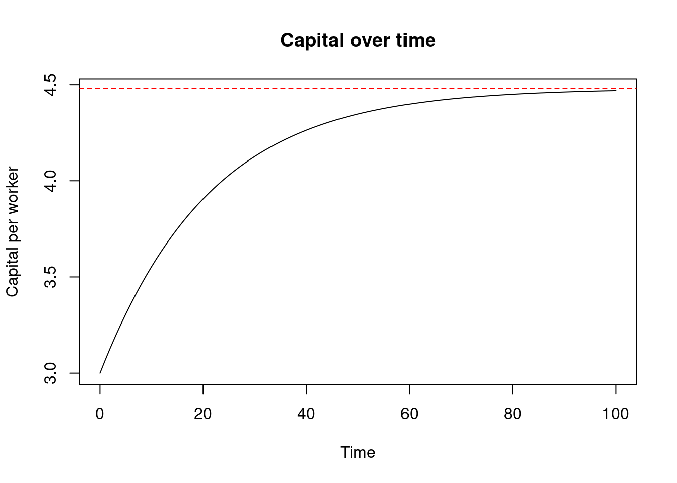
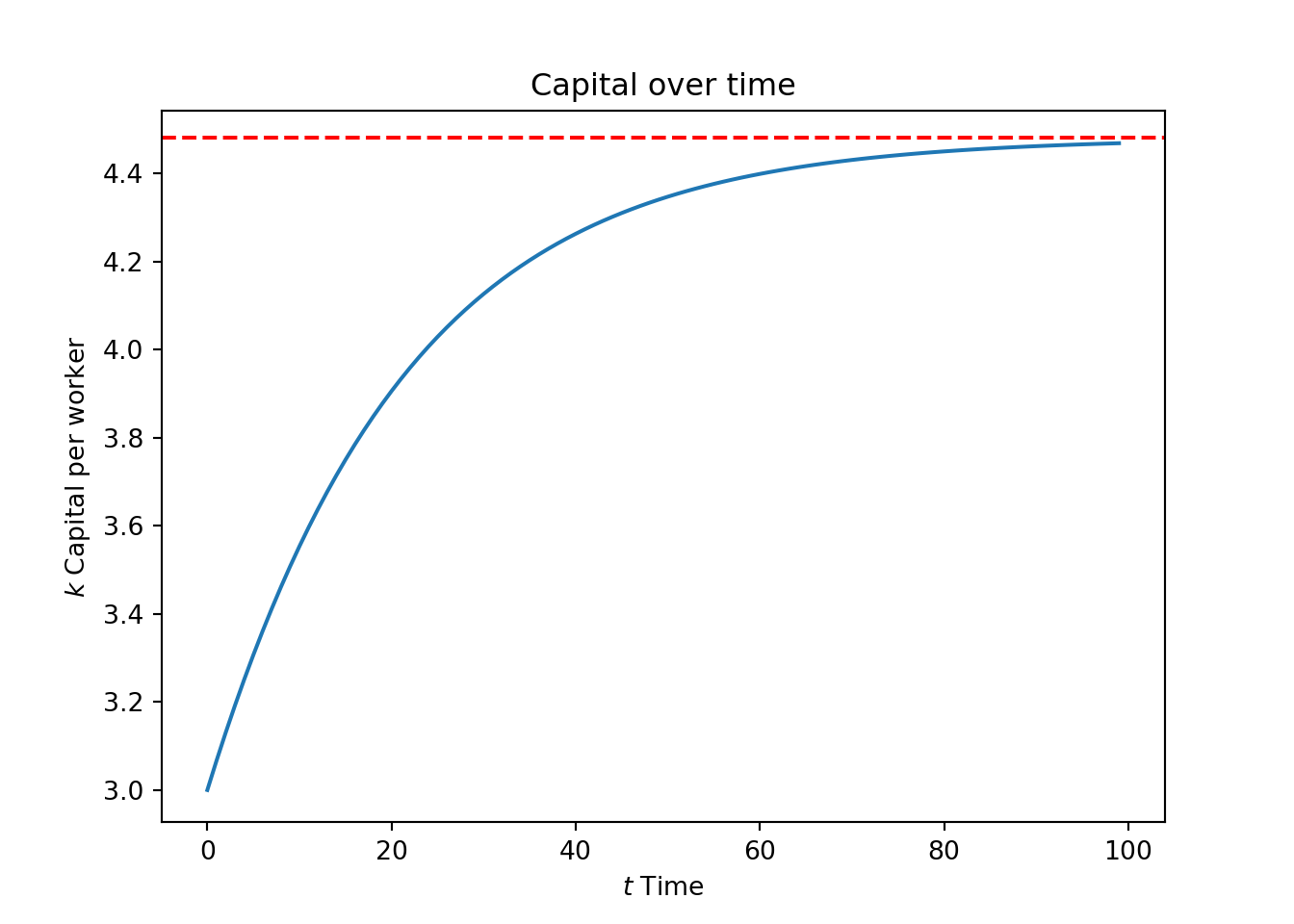
Print capital over time.

fig, ax = plt.subplots()
ax.plot(tv, kv)
ax.axhline(y=kstar, color='r', linestyle='--', label='Steady State')
ax.set_xlabel('$t$ Time')
ax.set_ylabel('$k$ Capital per worker')
ax.set_title('Capital over time')
plt.show()

# Plot capital over time
plot(tv, kv, type = "l", xlab = "Time", ylab = "Capital per worker",
     main = "Capital over time")
abline(h = kstar, col = "red", lty = 2)

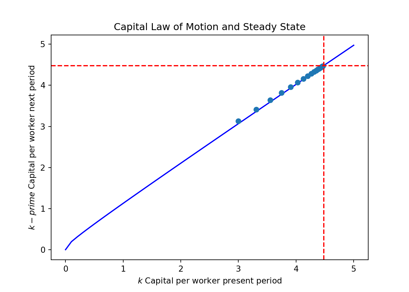
Print the per-capita law of motion and put the capital path into it.


kgridv=np.linspace(0,5,50);
knextv=f_kprime(kgridv);
fig, ax = plt.subplots()
ax.plot(kgridv, knextv, 'b-')
ax.plot(kv[0:-2:5], kprimev[1:-1:5], 'o')
ax.axhline(y=kstar, color='r', linestyle='--', label='Steady State')
ax.axvline(x=kstar, color='r', linestyle='--', label='Steady State')
ax.set_xlabel('$k$ Capital per worker present period')
ax.set_ylabel('$k-prime$ Capital per worker next period')
ax.set_title('Capital Law of Motion and Steady State')
plt.show()

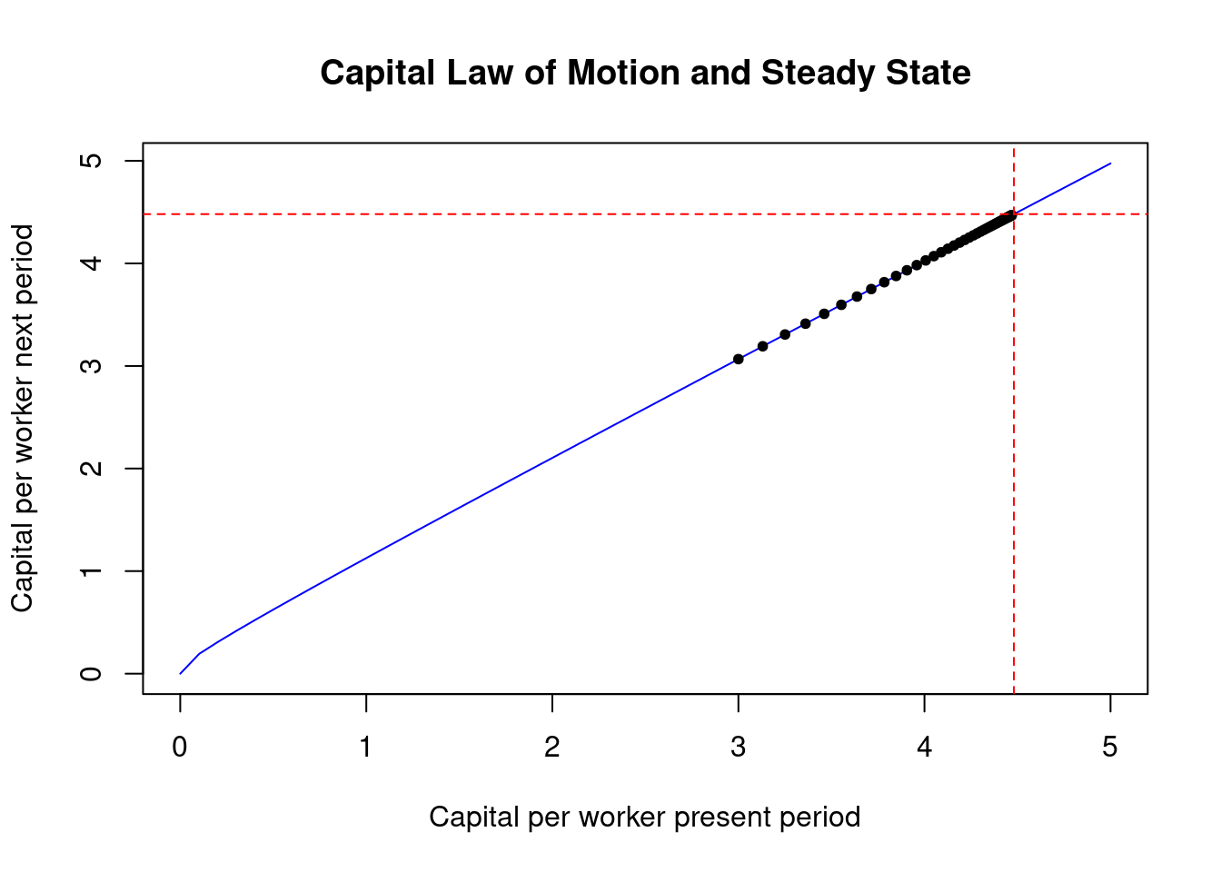
# Plot the per-capita law of motion and add the capital path to it
kgridv <- seq(0, 5, length.out = 50)
knextv <- f_kprime(kgridv)

plot(kgridv, knextv, type = "l", col = "blue", xlab = "Capital per worker present period",
     ylab = "Capital per worker next period", main = "Capital Law of Motion and Steady State")
points(kv[c(1:length(kv)-1) %% 2 == 0], kprimev[c(2:length(kprimev)) %% 2 == 0], col = "black", pch = 20)
abline(h = kstar, col = "red", lty = 2)
abline(v = kstar, col = "red", lty = 2)

This code will produce a plot showing the evolution of capital per worker over time and the horizontal line indicating the steady-state level of capital per worker.

Key Concepts and Summary
  • Solow growth model
  • Steady state
  • Balanced growth path